Hi Codeforces! I'm the author of the first two tasks in APIO 2018. Although the official site posted only the solution codes, I think the task analyses are equally appreciable, so I decided to publish them here.

Here's the link to the problem statements if you haven't seen them yet.

Problem A. New Home

Subtask 1

Naive solution will work.

Subtask 2

Simulate all the events (store open/store close/query) in chronological order. Maintain k BSTs, one per each (store-)type. During a query, for each type, check the two neighboring stores of the location. This solution runs in .

Subtask 3

Without the time constraint, the problem becomes querying the maximum of k distance functions, each of which is composed of some segments with slope  =  ± 1.

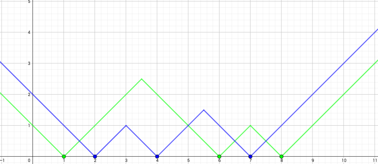
Fig. 1: Two types of stores locating at {1, 6, 8} and {2, 4, 7}

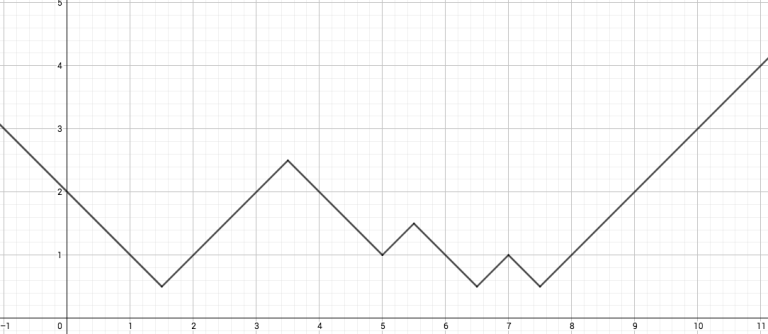
Fig. 2: The maximum of the two functions

The key here is to deal with the positive-slope and the negative-slope segments separately, and then combine their results afterwards. (Since they are symmetric, I'll just focus on the negative case.) There are many ways to do this (e.g. with segment tree/priority queue/BST/etc.), but the fastest and easiest way is to perform a mergesort-like scan for the queries and the segments from left to right.

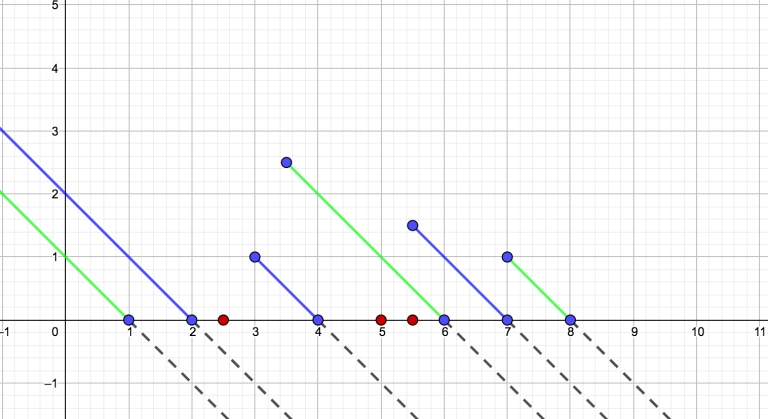
Fig. 3: The negative-slope segments from the previous example, with query points {2.5, 5, 5.5}. Note that we can let the segments extend below the x-axis (i.e. view them as rays), as this won't affect the correctness. This way, we only need to store one value (the x-intercept) when scanning and don't need to "pop" the segments.

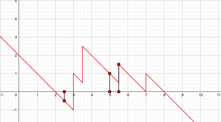
Fig. 4: The resulting (maximum) function. The query points yield result { - 0.5, 1, 1.5}.

So this subtask can be solved in .

Subtask 4

In this subtask, stores only get removed. When a store is removed, a partial upshift will occur in the distance function, and two new segments are generated.

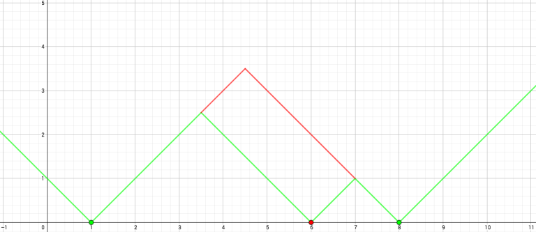
Fig. 5: Removing the red point results in the distance function’s partial upshift into two new segments.

Notice the new segments are always weakly higher than the old ones. Since we're calculating the maximum function, we don't have to remove the old segments (and/or their contributions) when adding in the new ones. Therefore, to answer a query, we can simply take into account all the segments added before it. This leads to a divide-and-conquer approach, where in each level, we use the previous mergesort-like method to calculate the segment-to-query contributions that cross mid-time. The naive implementation runs in , but can be easily improved to if the queries and segments are pre-sorted in spacial order. Another approach is to maintain along the x-axis a segment tree/BIT that stores the highest segment at a coordinate. This leads to a (or ) solution.

Subtask 5

There are (I know at least) two kinds of approaches to this subtask. The first kind is based on the classic "Number of Distinct Elements in an Interval" problem, which can be solved in . For each query, binary search the answer and solve the NDEI problem for the corresponding interval. This kind of solution runs in .

The second kind is based on sqrt decomposition. If we split the events (store open/store close/query) into chucks, since there are only O(C) types that are modified in the chunk, we can deal with the unmodified types with the Subtask 3 solution and modified types with Subtask 2. Depending on the implementation, this kind of solution runs in , , or O(n^1.5), and may require some parameter tuning.

Subtask 6

The key observation for this subtask is that when a store is inserted/removed, there are only O(1) new segments/rays created. This means that in total, there are at most O(n) different segments/rays, each having its own existing timeframe. We can use the "segment tree D&C" method to solve this. That is, we insert the segments/rays into a "time" segment tree, with its timeframe representing the "interval". And, each query is a leaf node in this "time" segment tree, so we run DFS on this tree while running Subtask 3 solution in each node to calculate the contributions. This solution runs in if the queries and segments are pre-sorted in spacial order. My implementation of this solution can be found in the APIO 2018 material package.

There are many variants of this solution. However, the ones are usually not fast enough, unless it has small constants.

Problem B. Circle Selection

Subtask 1

Naive solution will work. Note that the formula for circle intersection is (x_i - x_j)² + (y_i - y_j)² ≤ (r_i + r_j)².

Subtask 2

The problem becomes a one-dimensional interval-intersecting problem — c_i intersects with c_j iff [x_i - r_i, x_i + r_i] intersects with [x_j - r_j, x_j + r_j]. Therefore, we transform each circle into its corresponding interval. A handy property is that an eliminating interval is weakly larger than any of its corresponding eliminated intervals, so one of the endpoints of latter must lie in the former. With this in mind, we can do the procedure online with some interval querying data structure (e.g. segment tree/BST). This solution runs in .

Subtask 3

This subtask can be solved with the sweeping line technique. Say the line is horizontal (L: y = y₀) and moves downward (y₀↓). When the line meets a circle (y₀ = y_i + r_i), we put a "marker" at coordinate x = x_i on the line, and we remove the marker when the line leaves the circle (y₀ = y_i - r_i). It can be shown that if c_i intersects with c_j, there must be some instance y = y₀ *  such that and are adjacent. So we only need to check circle intersections between neighboring markers. If we maintain a BST of markers, we only need to check and when is inserted, and when is removed. This gives an solution.

Subtask 4

From now on, we will call the chosen circle in an iteration of the loop the eliminator, the corresponding eliminated circles eliminatees, and the action of plugging in information of two circles into the intersection formula to check intersection a query.

In a sense, it is quite silly for an eliminator to query distant circles, since only the nearby ones have chance of being removed. The problem here is how to systematically define “nearby”. My approach is to grid the plane into r-by-r unit squares, where r is the radius of the circles.

Property 1. The eliminatees’ origins must lie in the 5-by-5 region centered at the unit square containing the eliminator’s origin.

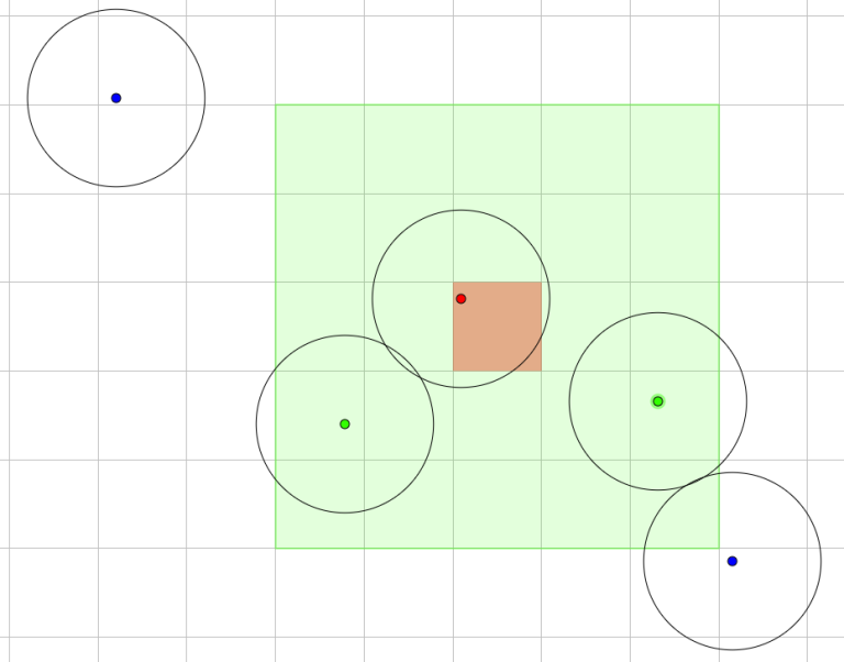
Fig. 6: An example showing Property 1. (Red origin = eliminator; Green origin = potential eliminatees; Blue origin = distant circles)

From Property 1, if we represent the grid as a 2D array having each element as a set of origins within the corresponding unit square, we only need to check at most 25 = O(1) sets of circles per eliminator. One may use hash table to implement this 2D array, but I used vector<vector<Point>>, with the first dimension be in discretized x-coordinate order and the second raw y-coordinate order. Under this implementation, we can access the 25 squares with binary search, so every loop iteration (in the problem description) can be done in , where z_i denotes the number of origins in the 5-by-5 region in that iteration, and the total time complexity is .

Property 2a. .

Proof. We calculate the sum from the perspective of an eliminatee. Note that for an eliminator to query the eliminatee, its origin must locate in the 5x5 region centered at the eliminatee's unit square.

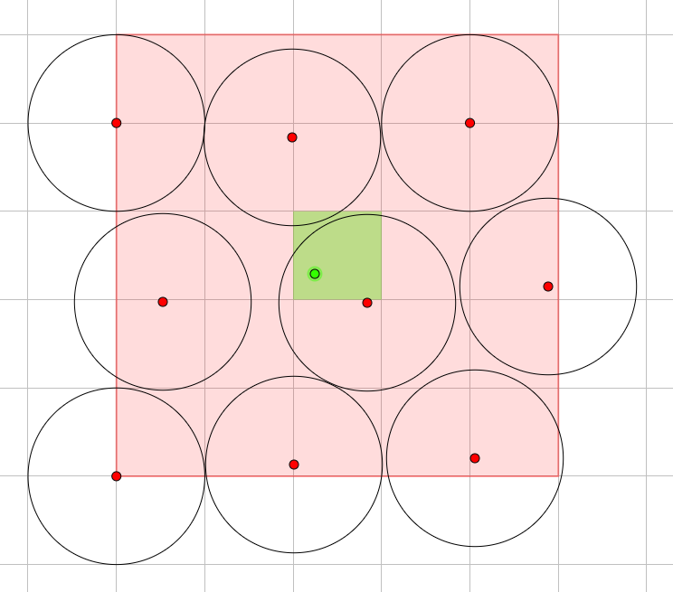
Fig 7: An eliminatee's origin and an example set of eliminators.

Property 3. The eliminators are disjoint. Property 4a. A 5x5 region contains at most O(1) disjoint unit circles.

So the sum is , and the total time complexity is .

Subtask 5 & 6

Unfortunately, Property 2a doesn’t apply to arbitrarily sized circles. But notice the size of the eliminators are weakly decreasing. If we start with square size = r_max², where r_max denotes the largest radius on the plane, the procedure will become more and more inefficient as r_max decreases. So when this radius becomes less then half of the gridding length, we split each unit square into four, halving the length.

Fig 8: When r_max becomes sufficiently small, we rescale the grid.

Since the gridding length  ≥  eliminator’s radius  ≥  eliminatees’ radius, Property 1 still holds. Therefore the time complexity of our new solution is , and because rescaling can be done in O(n) (by splitting an existing vector<Point> into two), the second term is .

Property 2b. .

Proof. Consider the eliminators with , where g denotes the gridding length.

Property 3. The eliminators are disjoint. Property 4b. A 5x5 region contains at most O(1) disjoint at-least-half-unit circles.

So the contribution of the same-ordered eliminators is O(n). There are different orders, therefore the sum, and the final time complexity is . Again, you can find my implementation in the APIO 2018 material package.