


Hi all,
I would like to share with you a part of my undergraduate thesis on a Multi-String Pattern Matcher data structure. In my opinion, it's easy to understand and hard to implement correctly and efficiently. It's competitive against other MSPM data structures (Aho-Corasick, suffix array/automaton/tree to name a few) when the dictionary size is specifically (uncommonly) large.
I would also like to sign up this entry to bashkort's Month of Blog Posts:-)
Abstract
This work describes a hash-based mass-searching algorithm, finding (count, location of first match) entries from a dictionary against a string $$$s$$$ of length $$$n$$$. The presented implementation makes use of all substrings of $$$s$$$ whose lengths are powers of $$$2$$$ to construct an offline algorithm that can, in some cases, reach a complexity of $$$O(n \log^2n)$$$ even if there are $$$O(n^2)$$$ possible matches. If there is a limit on the dictionary size $$$m$$$, then the precomputation complexity is $$$O(m + n \log^2n)$$$, and the search complexity is bounded by $$$O(n\log^2n + m\log n)$$$, even if it performs in practice like $$$O(n\log^2n + \sqrt{nm}\log n)$$$. Other applications, such as finding the number of distinct substrings of $$$s$$$ for each length between $$$1$$$ and $$$n$$$, can be done with the same algorithm in $$$O(n\log^2n)$$$.
Problem Description
We want to write an offline algorithm for the following problem, which receives as input a string $$$s$$$ of length $$$n$$$, and a dictionary $$$ts = \{t_1, t_2, .., t_{\lvert ts \rvert}\}$$$. As output, it expects for each string $$$t$$$ in the dictionary the number of times it is found in $$$s$$$. We could also ask for the position of the fist occurrence of each $$$t$$$ in $$$s$$$, but the paper mainly focuses on the number of matches.
Algorithm Description
We will build a DAG in which every node is mapped to a substring from $$$s$$$ whose length is a power of $$$2$$$. We will draw edges between any two nodes whose substrings are consecutive in $$$s$$$. The DAG has $$$O(n \log n)$$$ nodes and $$$O(n \log^2 n)$$$ edges.
We will break every $$$t_i \in ts$$$ down into a chain of substrings of $$$2$$$-exponential length in strictly decreasing order (e.g. if $$$\lvert t \rvert = 11$$$, we will break it into $$$\{t[1..8], t[9..10], t[11]\}$$$). If $$$t_i$$$ occurs $$$k$$$ times in $$$s$$$, we will find $$$t_i$$$'s chain $$$k$$$ times in the DAG. Intuitively, it makes sense to split $$$s$$$ like this, since any chain has length $$$O(\log n)$$$.
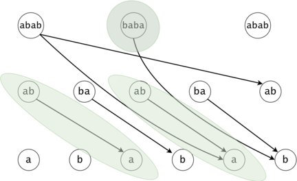
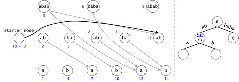
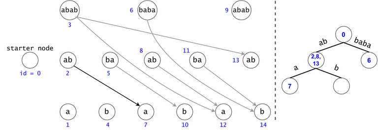
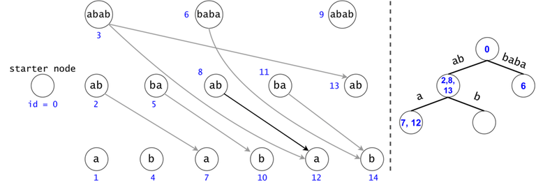
Figure 1: The DAG for $$$s = (ab)^3$$$. If $$$ts = \{aba, baba, abb\}$$$, then $$$t_0 = aba$$$ is found twice in the DAG, $$$t_1 = baba$$$ once, and $$$t_2 = abb$$$ zero times.
Redundancy Elimination: Associated Trie, Tokens, Trie Search
A generic search for $$$t_0 = aba$$$ in the DAG would check if any node marked as $$$ab$$$ would have a child labeled as $$$a$$$. $$$t_2 = abb$$$ is never found, but a part of its chain is ($$$ab$$$). We have to check all $$$ab$$$s to see if any may continue with a $$$b$$$, but we have already checked if any $$$ab$$$s continue with an $$$a$$$ for $$$t_0$$$, making second set of checks redundant.
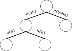
Figure 2: If the chains of $$$t_i$$$ and $$$t_j$$$ have a common prefix, it is inefficient to count the number of occurrences of the prefix twice. We will put all the $$$t_i$$$ chains in a trie. We will keep the hashes of the values on the trie edges.
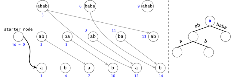
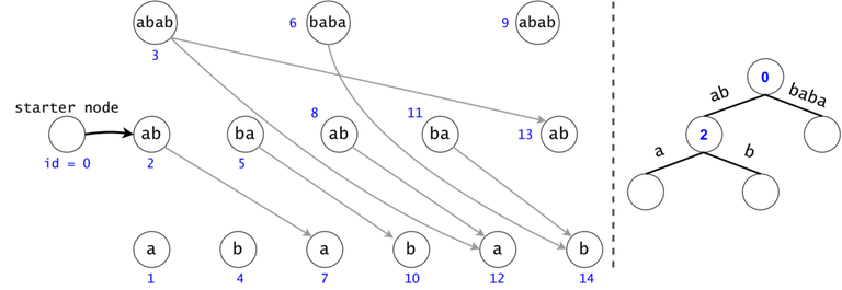
In order to generalize all of chain searches in the DAG, we will add a starter node that points to all other nodes in the DAG. Now all DAG chains begin in the same node.
The actual search will go through the trie and find help in the DAG. The two Data Structures cooperate through tokens. A token is defined by both its value (the DAG index in which it’s at), and its position (the trie node in which it’s at).
Token count bound and Token propagation complexity
Property 1: There is a one-to-one mapping between tokens and $$$s$$$’ substrings. Any search will generate $$$O(n^2)$$$ tokens.
Proof 1: If two tokens would describe the same substring of $$$s$$$ (value-wise, not necessarily position-wise), they would both be found in the same trie node, since the described substrings result from the concatenation of the labels on the trie paths from the root.
Now, since the two tokens are in the same trie node, they can either have different DAG nodes attached (so different ids), meaning they map to different substrings (i.e. different starting positions), or they belong to the same DAG node, so one of them is a duplicate: contradiction, since they were both propagated from the same father.
As a result, we can only generate in a search as many tokens as there are substrings in $$$s$$$, $$$n(n+1)/2 + 1$$$, also accounting for the empty substring (Starter Node's token). $$$\square$$$
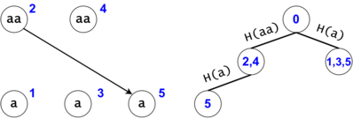
Figure 3: $$$s = aaa, ts = \{a, aa, aaa\}$$$. There are two tokens that map to the same DAG node with the id $$$5$$$, but they are in different trie nodes: one implies the substring $$$aaa$$$, while the other implies (the third) $$$a$$$.
Property 2: Ignoring the Starter Node's token, any token may divide into $$$O(\log n)$$$ children tokens. We can propagate a child in $$$O(1)$$$ (the cost of the membership test (in practice, against a hashtable containing rolling hashes passed through a Pseudo-Random Function)).
As a result, we have a pessimistic bound of $$$O(n^2 \log n)$$$ for a search.
Another redundancy: DAG suffix compression
Property 3: If we have two different tokens in the same trie node, but their associated DAG nodes’ subtrees are identical, it is useless to propagate the second token anymore. We should only propagate the first one, and count twice any finding that it will have.
Proof 3: If we don’t merge the tokens that respect the condition, their children will always coexist in any subsequent trie nodes: if one gets propagated, the other will as well, or none get propagated. We can apply this recursively to cover the entire DAG subtree. $$$\square$$$
Intuitively, we can consider two tokens to be the same if their future cannot be different, no matter their past.
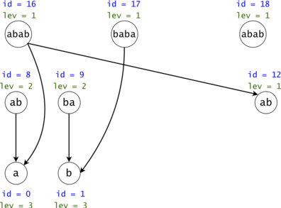
Figure 4: The DAG from Figure 1 post suffix compression. We introduce the notion of leverage. If we compress $$$k$$$ nodes into each other, the resulting one will have a leverage equal to $$$k$$$. We were able to compress two out of the three $$$ab$$$ nodes. If we are to search now for $$$aba$$$, we would only have to only propagate one token $$$ab \rightarrow a$$$ instead of the original two.
Property 4: The number of findings given by a compressed chain is the minimum leverage on that chain (i.e. we found $$$bab$$$ $$$\min([2, 3]) = 2$$$ times, or $$$ab$$$ $$$\min([2]) + \min([1]) = 3$$$ times). Also, the minimum on the chain is always given by the first DAG node on the chain (that isn't the Starter Node).
Proof 4: Let $$$ch$$$ be a compressed DAG chain. If $$$1 \leq i < j \leq \lvert ch \rvert$$$, then $$$node_j$$$ is in $$$node_i$$$'s subtree. The more we go into the chain, the less restrictive the compression requirement becomes (i.e. fewer characters need to match to unite two nodes).
If we united $$$node_i$$$ with another node $$$x$$$, then there must be a node $$$y$$$ in $$$x$$$'s subtree that we can unite with $$$node_j$$$. Therefore, $$$lev_{node_i} \leq lev_{node_j}$$$, so the minimum leverage is $$$lev_{node_1}$$$. $$$\square$$$
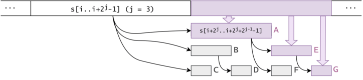
Figure 5: Practically, we compress nodes with the same subtree hash. Notice that the subtree of a DAG node is composed of characters that follow sequentially in $$$s$$$.
Remark: While the search complexity for the first optimization (adding the trie) isn't too difficult to point down, the second optimization (the more powerful DAG compression) is much harder to work with: the worst case is much more difficult to find (the compression obviously has been specifically chosen to move away the worst case))).
Complexity computation: without DAG compression
We will model a function $$$NT : \mathbb{N}^* \rightarrow \mathbb{N}, NT(m) = $$$ if the dictionary character count is at most $$$m$$$, what is the maximum number of tokens that we can generate?
Property 5: If $$$t'$$$ cannot be found in $$$s$$$, let $$$t$$$ be its longest prefix that can be found in $$$s$$$. Then, no matter if we would have $$$t$$$ or $$$t'$$$ in any $$$ts$$$, the number of generated tokens would be the same. As a result, we would prefer adding $$$t$$$, since it would increase the size of the dictionary by a smaller amount. This means that in order to maximize $$$NT(m)$$$, we would include only substrings of $$$s$$$ in $$$ts$$$.
If $$$l = 2^{l_1} + 2^{l_2} + 2^{l_3} + ... + 2^{l_{last}}$$$, with $$$l_1 > l_2 > l_3 > ... > l_{last}$$$, then we can generate at most $$$\Sigma_{i = 1}^{last} n+1 - 2^{l_i}$$$ tokens by adding all possible strings of length $$$l$$$ into $$$ts$$$. However, we can add all tokens by using only one string of length $$$l$$$ if $$$s = a^n$$$ and $$$t = a^l$$$.
As a consequence, the upper bound if no DAG compression is performed is given by the case $$$s = a^n$$$, with $$$ts$$$ being a subset of $$${a^1, a^2, .., a^n}$$$.
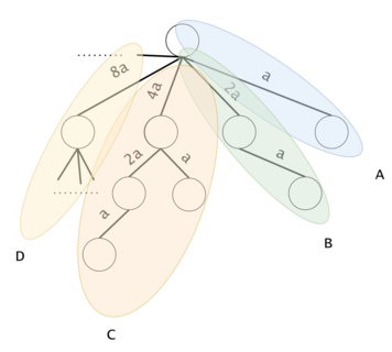
Figure 6: Consider the "full trie" to be the complementary trie filled with all of the options that we may want to put in $$$ts$$$. We will segment it into sub-tries. Let $$$ST(k)$$$ be a sub-trie containing the substrings $$${a^{2^k}, .., a^{2^{k+1}-1}} \,\, \forall \, k \geq 0$$$. The sub-tries are marked here with A, B, C, D, ...}
Property 6: Let $$$1 \leq x = 2^{x_1} + .. + 2^{x_{last}} < y = x + 2^{y_1} + .. + 2^{y_{last}} \leq n$$$, with $$$2^{x_{last}} > 2^{y_1}$$$. We will never hold both $$$a^x$$$ and $$$a^y$$$ in $$$ts$$$, because $$$a^y$$$ already accounts all tokens that could be added by $$$a^x$$$: $$$a^x$$$'s chain in the full trie is a prefix of $$$a^y$$$'s chain.
We will devise a strategy of adding strings to an initially empty $$$ts$$$, such that we maximize the number of generated tokens for some momentary values of $$$m$$$. We will use two operations:
- upgrade: If $$$x < y$$$ respect Property 6, $$$a^x \in ts,\, a^y \notin ts$$$, then replace $$$a^x$$$ with $$$a^y$$$ in $$$ts$$$.
- add: If $$$a^y \notin ts$$$, and $$$\forall \, a^x \in ts$$$, we can't upgrade $$$a^x$$$ to $$$a^y$$$, add $$$a^y$$$ to $$$ts$$$.
Property 7: If we upgrade $$$a^x$$$, we will add strictly under $$$x$$$ new characters to $$$ts$$$, since $$$2^{y_1} + .. + 2^{y_{last}} < 2 ^ {x_{last}} \leq x$$$.
Property 8: We don't lose optimality if we only use add for only $$$y$$$s that are powers of two. If $$$y$$$ isn't a power of two, we can use add on the most significant power of two of $$$y$$$, then upgrade it to the full $$$y$$$.
Property 9: We also don't lose optimality if we upgrade from $$$a^x$$$ to $$$a^y$$$ only if $$$y - x$$$ is a power of two (let this be called minigrade). Otherwise, we can upgrade to $$$a^y$$$ by a sequence of minigrades.
Statement 10: We will prove by induction that (optimally) we will always exhaust all upgrade operations before performing an add operation.
Proof 10: We have to start with an add operation. The string that maximizes the number of added tokens ($$$n$$$) also happens to have the lowest length ($$$1$$$), so we will add $$$a^1$$$ to $$$ts$$$. Notice that we have added/upgraded all strings from sub-trie $$$ST(0)$$$, ending the first step of the induction.
For the second step, assume that we have added/upgraded all strings to $$$ts$$$ from $$$ST(0), .., ST(k-1)$$$, and we want to prove that it's optimal to add/upgrade all strings from $$$ST(k)$$$ before exploring $$$ST(k+1), ...$$$.
By enforcing Property 8, the best string to add is $$$a^{2^k}$$$, generating the most tokens, while being the shortest remaining one.
| operation | token gain | |ts| gain |
|---|---|---|
| add $$$a^{2^{k+1}}$$$ | $$$n+1 - 2^{k+1}$$$ | $$$2^{k+1}$$$ |
| any minigrade | $$$\geq n+1 - (2^{k+1}-1)$$$ | < $$$2^k$$$ |
Afterwards, we gain more tokens by doing any minigrade on $$$ST(k)$$$, while increasing $$$m$$$ by a smaller amount than any remaining add operation. Therefore, it's optimal to first finish all minigrades from $$$ST(k)$$$ before moving on. $$$\square$$$
We aren't interested in the optimal way to perform the minigrades. Now, for certain values of $$$m$$$, we know upper bounds for $$$NT(m)$$$:
| subtries in ts | m | NT(m) |
|---|---|---|
| $$$ST(0)$$$ | $$$1$$$ | $$$n$$$ |
| $$$ST(0), ST(1)$$$ | $$$1+3$$$ | $$$n + (n-1) + (n-2)$$$ |
| $$$ST(0), .., ST(2)$$$ | $$$1+3+(5+7)$$$ | $$$n + ... + (n-6)$$$ |
| $$$ST(0), .., ST(3)$$$ | $$$1+3+(5+7)+(9+11+13+15)$$$ | $$$n + ... + (n-14)$$$ |
| ... | ||
| $$$ST(0), .., ST(k-1)$$$ | $$$1+3+5+7+...+(2^k-1) = 4^{k-1}$$$ | $$$n + ... + (n+1 - (2^k-1))$$$ |
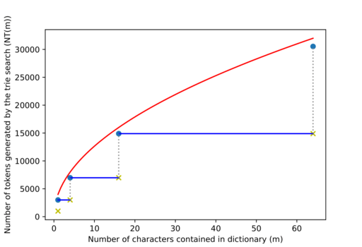
Figure 7: The entries in the table are represented by goldenrod crosses.
We know that if $$$m \leq m'$$$, then $$$NT(m) \leq NT(m')$$$, so we'll upper bound $$$NT$$$ by forcing $$$NT(4^{k-2}+1) = NT(4^{k-2}+2) = ... = NT(4^{k-1}) \,\, \forall \, k \geq 2$$$ (represented with blue segments in figure 7. We will also assume that the goldenrod crosses are as well on the blue lines, represented here as blue dots.
We need to bound:
But if $$$m = 4^{k-1} \Rightarrow 2^{k+1} = 4 \sqrt m \Rightarrow NT(m) \leq n + 4 n \sqrt m$$$.
So the whole $$$NT$$$ function is bounded by $$$NT(m) \leq n + 4 n \sqrt m$$$, the red line in figure 7. $$$NT(m) \in O(n \sqrt m)$$$.
The total complexity of the search part is now also bounded by $$$O(n \sqrt m \log n)$$$, so the total program complexity becomes $$$O(m + n \log^2 n + \min(n \sqrt m \log n, n^2 \log n))$$$.
Corner case Improvement
We will now see that adding the DAG suffix compression moves the worst case away from $$$s = a^n$$$ and $$$ts = \{a^1, .., a^n\}$$$. We will prove that the trie search complexity post compression for $$$s = a^n$$$ is $$$O(n \log^2n)$$$.
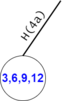
Figure 8: A trie node's "father edge" unites it with its parent in the trie.
Statement 11: If a trie node’s "father edge" is marked as $$$a^{2^x}$$$, then there can be at most $$$2^x$$$ tokens in that trie node.
Proof 11: If the "father edge" is marked as $$$a^{2^x}$$$, then any token in that trie node can only progress for at most another $$$2^x-1$$$ characters in total. For example, in figure 8, a token can further progress along its path for at most another three characters, possibly going through $$$a^2$$$ and $$$a$$$.
Since all characters are $$$a$$$ here, the only possible DAG subtree configurations accessible from this trie node are the ones formed from the substrings $$${a^0, a^1, a^2, a^3, ..., a^{2^x-1}}$$$, so $$$2^x$$$ possible subtrees (figure 9).
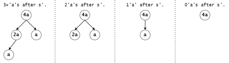
Figure 9: For example, consider a token's associated DAG node with the value of $$$a^4$$$, and $$$s'$$$ to be the substring that led to that trie node (i.e. the concatenation of the labels on the trie path from the root).
If we have more than $$$2^x$$$ tokens in the trie node, then there must exist two tokens who belong to the same DAG subtree configuration, meaning that their nodes would have been united during the compression phase. Therefore, we can discard one of them.
So the number of tokens in a trie node cannot be bigger than the number of distinct subtrees that can follow from the substring that led to that trie node (in this case $$$2^x$$$). $$$\square$$$
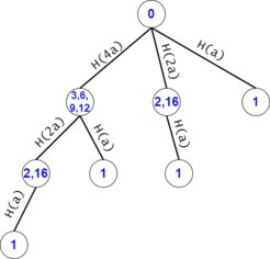
Figure 10: For example, the trie search after the DAG compression for $$$s = a^7$$$, $$$ts = {a^1, a^2, .., a^7}$$$.
Let $$$trie(n)$$$ be the trie built from the dictionary $$${a^1, a^2, a^3, ..., a^n}$$$.
Let $$$cnt_n(2^x)$$$ be the number of nodes in $$$trie(n)$$$ that have their "father edge" labeled as $$$a^{2^x}$$$. For example, in figure 10, $$$cnt_7(2^0) = 2^2$$$, $$$cnt_7(2^1) = 2^1$$$, and $$$cnt_7(2^2) = 2^0$$$.
Pick $$$k$$$ such that $$$2^{k-1} \leq n < 2^k$$$. Then, $$$trie(n) \subseteq trie(2^k-1)$$$. $$$trie(2^k-1)$$$ would generate at least as many tokens as $$$trie(n)$$$ during the search.
Statement 12: We will prove by induction that $$$trie(2^k-1)$$$ has $$$cnt_{2^k-1}(2^x) = 2^{k-1-x} \,\, \forall \, x \in [0, k-1]$$$.
Proof 12: If $$$k = 1$$$, then $$$trie(1)$$$ has only one outgoing edge from the root node labeled $$$a^1 \Rightarrow cnt_1(2^0) = 1 = 2^{1-1-0}$$$.
We will now suppose that we have proven this statement for $$$trie(2^{k-1}-1)$$$ and we will try to prove it for $$$trie(2^k-1)$$$.
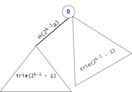
Figure 11: The expansion from $$$trie(2^{k-1}-1)$$$ to $$$trie(2^k-1)$$$.
As a result:
- $$$cnt_{2^k-1}(1) = 2 \cdot cnt_{2^{k-1}-1}(1) = 2^{k-2} \cdot 2 = 2^{k-1}$$$,
- $$$cnt_{2^k-1}(2) = 2 \cdot cnt_{2^{k-1}-1}(2) = 2^{k-2}$$$,
- ...
- $$$cnt_{2^k-1}(2^{k-2}) = 2 \cdot cnt_{2^{k-1}-1}(2^{k-2}) = 2^1$$$,
- $$$cnt_{2^k-1}(2^{k-1}) = 1 = 2^0. \,\, \square$$$
We will now count the number of tokens for $$$trie(2^k-1)$$$:
So there are $$$O(k \cdot 2^{k-1})$$$ tokens in $$$trie(2^k-1)$$$. Since $$$2^{k-1} \leq n < 2^k \Rightarrow k-1 \leq \log_{2}n < k \Rightarrow k \leq \log_{2}n+1$$$.
Therefore, $$$2^{k-1} \leq n \Rightarrow O(k \cdot 2^{k-1}) \subset O((\log_{2}n + 1) \cdot n) = O(n \log n)$$$, so for $$$s = a^n$$$, its associated trie search will generate $$$O(n \log n)$$$ tokens, and the trie search will take $$$O(n\log^2n)$$$.
We can fit the entire program's complexity in $$$O(n\log^2n)$$$ if we give the dictionary input directly in hash chain form.
Complexity computation: with DAG compression
This is the most important part of the blog. We will use the following definitions:
If $$$\lvert t \rvert = 2^{k_1} + 2^{k_2} + 2^{k_3} + ... + 2^{k_{last}}$$$, with $$$k_1 > k_2 > k_3 > ... > k_{last}$$$, then let $$$get(t, i) = t[2^{k_1} + 2^{k_2} + .. + 2^{k_{i-1}} : 2^{k_1} + 2^{k_2} + .. + 2^{k_{i}}], i \geq 1$$$. For example, if $$$t = ababc$$$, $$$get(t, 1) = abab, get(t, 2) = c$$$.
Similarly, if $$$p = 2^{k_1} + 2^{k_2} + .. + 2^{k_{last}}$$$, let $$$LSB(p) = 2^{k_{last}}$$$.
If $$$t$$$ is a substring of $$$s$$$, and we know $$$t$$$'s position in $$$s$$$ ($$$t = s[i..j]$$$), then let $$$shade(s, t) = s[i.. \min(n, j+LSB(j-i+1)-1)]$$$ (i.e. the shade of $$$t$$$ is the content of its DAG node subtree). For example, if $$$s = asdfghjkl$$$, $$$shade(s, sdfg) = sdfg + hjk$$$, $$$shade(s, a) = a$$$, $$$shade(s, jk) = jk + l$$$, $$$shade(s, jkl) = jkl$$$. A shade that prematurely ends (i.e. if $$$n$$$ would be larger, the shade would be longer) may be ended with $$$\varnothing$$$: $$$shade(s, kl) = kl\varnothing$$$.
Let $$$sub(s, t)$$$ denote the number of node chains from $$$s$$$' DAG post-compression whose values are equal to $$$t$$$. For example, $$$sub(abababc, ab) = 2$$$. Notice that $$$sub(s, t)$$$ is equal to the number of distinct values that $$$shade(s, t)$$$ takes.
Let $$$popcount(p)$$$ be the number of bits equal to 1 in $$$p$$$'s representation in base 2.
Statement 13: We choose to classify the trie search tokens in two categories: tokens that are alone (or not alone) in their trie nodes. An alone token describes a distinct substring of $$$s$$$. Thus, it can only have alone tokens as children (their substring equivalent having a distinct prefix of $$$s$$$). We can easily find decent bounds for the number of alone tokens depending of $$$m$$$. We will shortly see that the maximum number of non-alone tokens is relatively small and is independent of $$$m$$$.
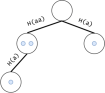
Figure 12: For example, $$$s = a^3$$$ generates two non-alone tokens (for the two $$$a^2$$$s) and two alone tokens (for $$$a^3$$$ and the $$$a$$$ s), not counting the starter node's token.
Statement 14: There are at most $$$O(m)$$$ alone tokens in the trie.

Figure 13: Any $$$t_i$$$ can add at most $$$O(popcount(length(t_i)))$$$ alone tokens in the trie.
Proof 14: For each string in the dictionary, let $$$z_i = \lvert t_i \rvert \,\, \forall \, 1 \leq i \leq \lvert ts \rvert$$$, and $$$z_i = 0 \,\, \forall \, \lvert ts \rvert < i \leq m$$$.
The maximum number of alone tokens in the trie is:
But $$$\Sigma_{i=1}^{m} popcount(z_i) \leq \Sigma_{i=1}^{m} z_i = m$$$, achievable when $$$z_i = 1 \,\, \forall \, 1 \leq i \leq m$$$. $$$\square$$$
The bound is tight for practical values of $$$n$$$ (e.g. generate $$$s$$$ with $$$n = 10^8$$$ such that all substrings of size $$$7$$$ are distinct: $$$\lvert \Sigma \rvert ^ {7} \gg n$$$, even for $$$\lvert \Sigma \rvert = 26$$$. Take $$$ts$$$ to be all $$$s$$$' substrings of size $$$7$$$. Each $$$t$$$ will add at least one alone token, for approximately $$$m/7$$$ alone tokens in total).
Theorem 15: The maximum number of non-alone tokens is $$$O(n \log n)$$$.
Proof 15: Let the number of non-alone tokens generated by $$$s$$$ (considering that $$$ts$$$ contains every substring of $$$s$$$) to be noted with $$$NTna(s)$$$. Also, let the number of alone tokens be noted with $$$NTa(s)$$$: $$$NTna(s) + NTa(s) = NT(s)$$$ (note that we overloaded $$$NT$$$ here).
For example, $$$\max(NTna(s) \mid \lvert s \rvert = 3) = 2$$$, achieved for $$$s = a^3$$$. For longer lengths, there are many patterns that can achieve $$$NTNa(s) \in O(n \log n)$$$, such as $$$a^n$$$, $$$(ab)^k$$$, $$$(ab..z)^k$$$, $$$a^kba^{k-1}ba^{k-2}b...$$$, etc.
We will now redefine the problem of counting the number of non-alone tokens such that it no longer implies a trie search: for a string $$$s$$$, count the substrings $$$t$$$ of $$$s$$$ for which $$$sub(s, t) > 1$$$.
For example, for $$$s = a^3$$$, we won't count the substring $$$a^3$$$ because $$$sub(s, a^3) = 1$$$. We will count both $$$a^2$$$s ($$$s[1 .. 2]$$$ and $$$s[2 .. 3]$$$) because $$$sub(s, a^2) = 2$$$. We won't count any of the $$$a$$$s because they all have the same shade: $$$sub(s, a) = 1$$$. We arrive at $$$NTna(a^3) = 2$$$.
Property 16: Any string $$$s$$$ can be written in the following form: $$$s = s_1^{a_1}s_2^{a_2}s_3^{a_3}...s_k^{a_k}$$$, with $$$s_i \in \Sigma$$$, $$$a_i \geq 1 \,\, \forall \, 1 \leq i \leq k$$$. Also, we choose the representation such that $$$s_i \neq s_{i+1} \,\, \forall \, 1 \leq i < k$$$.
Let $$$f(n) = \max (NTna(s) \mid \lvert s \rvert = n)$$$. We will find a limit for $$$f(n)$$$ through recurrence.
We will split a given $$$s$$$ in two parts: $$$s = s_1^{a_1} + s_2^{a_2}s_3^{a_3}...s_k^{a_k}$$$.
Property 17: $$$NTna(s) \leq NTna(s_1^{a_1}) + 2NTa(s_1^{a_1}) + NTna(s_2^{a_2}s_3^{a_3}...s_k^{a_k}) + 2 \,\, \cdot $$$ the contribution of the substrings that begin in the left hand side (in the first $$$a_1$$$ characters) and end in the right hand side (not in the first $$$a_1$$$ characters).
Proof 17: We will start with $$$s_2^{a_2}s_3^{a_3}...s_k^{a_k}$$$ and build $$$s$$$ by adding $$$s_1^{a_1}$$$ as a prefix. Let $$$S_1$$$ and $$$S_2$$$ be two substrings that are fully contained within $$$s[:a_1]$$$ (i.e. in $$$s_1^{a_1}$$$). We are interested in how do the shades of $$$S_1$$$ and $$$S_2$$$ change post-union with $$$s_2^{a_2}... \,$$$ (can the shades become different if they were equal, or the opposite):
If the shades of $$$S_1$$$ and $$$S_2$$$ are different from the start:
- If exactly one of them prematurely ends (i.e. $$$s_1^{a_1} = a^3$$$, $$$shade(s_1^{a_1}, s_1^{a_1}[1..2]) = a^3$$$, $$$shade(s_1^{a_1}, s_1^{a_1}[2..3]) = a^2\varnothing$$$), then the incomplete shade will contain $$$s_2$$$, which cannot be found in the previously complete shade, which only contains $$$s_1 \neq s_2$$$.
- If both shades prematurely end, then both will look like $$$s_1^?s_2...$$$, but $$$s_2$$$ must occur at different points (because the shades are different, only contain $$$s_1$$$ and end prematurely).
- If no shade prematurely ends, then they cannot be altered post-unite, so the equality status between the shades doesn't change.
If $$$shade(s[:a_1], S_1) = shade(s[:a_1], S_2)$$$, then $$$S_1 = S_2$$$.
- If both shades prematurely end, then $$$S_1$$$ and $$$S_2$$$ describe the same substring, contradiction.
- If no shade prematurely ends, then they cannot be altered post-unite, so the equality status between the shades doesn't change.
- If exactly one shade prematurely ends, then the shades aren't identical, contradiction.
Since the relation between the shades of $$$S_1$$$ and $$$S_2$$$ doesn't change post-appending $$$s_1^{a_1}$$$ to $$$s_2^{a_2}s_3^{a_3}...s_k^{a_k}$$$ for no pair $$$(S_1, S_2)$$$, we can add $$$NTna(s_1^{a_1})$$$ to $$$NTna(s_2^{a_2}s_3^{a_3}...s_k^{a_k})$$$.
However, there may exist "dormant" substrings in $$$s_2^{a_2}...$$$ (i.e. substrings $$$u$$$ for which $$$sub(s_2^{a_2}..., u) = 1$$$, and post-unite $$$sub(s_1^{a_1}s_2^{a_2}..., u) > 1$$$ since $$$u$$$ also exists in $$$s_1^{a_1}$$$ with a different shade, meaning that we have to add $$$1$$$ from behind). As a result, $$$s_1^{a_1}$$$'s alone tokens may become non-alone for $$$s$$$, so we have to count them twice ($$$2NTa(s_1^{a_1})$$$) in order to bound $$$NTna(s)$$$.
A substring of $$$s$$$ that begins in $$$s_1^{a_1}$$$ and ends in $$$s_2^{a_2}...\,$$$ contributes if we can find it again in $$$s$$$, with a different shade. If we can't find it, its associated token is alone for now (dormant). Similarly, we have to double all findings to bound, since each could correspond to a dormant substring from $$$s_2^{a_2}...\,$$$. $$$\square$$$


