Recently, I was asked to help flesh out a problem for the NAIPC 2019 contest whose problems are also used every year as the "Grand Prix of America". Although I didn't invent this problem, I helped write a solution and create some of the test data for Problem C, Cost Of Living.

From the problem setter's perspective, this was intended to be an easy, A-level problem: suppose you have an table of values a_y, c that meet the condition that: for some m_c > 0.

If you are given a subset of the values in this table, and a subset of the values for i_k, determine whether a set of queried values a_y', c' is uniquely determined or not. Note that a_0, c = b_c.

Most contestants immediately realized that above product can be written as a sum by taking the logarithm:

Each given value thus represents a linear equation in unknowns , , and (plus some trivial equations for the subset of i_k that may be given. On the right hand side of the system appear the logarithms of the given table values. The left hand side of the system has only integer coefficients. Each row contains y + 1 1's and one coefficient with value y.

Each query, in turn, can also be written as a linear equation by introducing a variable :

Now, all that is left is to solve for the query variables using a traditional method (Gaussian Elimination with partial pivoting) and report the results — or so we thought.

While top teams disposed of this problem quickly, there was a great deal of uncertainty among some contestants whether this approach would work. One team attempted to solve the problem with a homegrown variant of Gaussian elimination, but got WA because their answer was too far off the requested answer (the answer had to be given with 1e-4 rel tolerance in this problem).

When they downloaded the judge data generator scripts, they observed that the amount of error in their implementation changed when they printed the input data with higher precision, which was very confusing to them.

For this problem, the input data was not given with full precision because it involves products with up to 20 factors. For instance, if b_c = m_c = i_k = 1.1 than a_10, c = 6.72749994932560009201 (exactly) but the input data would be rounded to 6.7274999493. If they changed this and printed instead 6.72749994932561090621, their solution would be much closer to the expected answer. Their result became even better when they used a floating point number type that uses more bits internally, such as quad-precision floats or java.math.BigDecimal. Thus, they concluded, they were doomed to be begin with because the input data was broken.

What could account for this phenomenon?

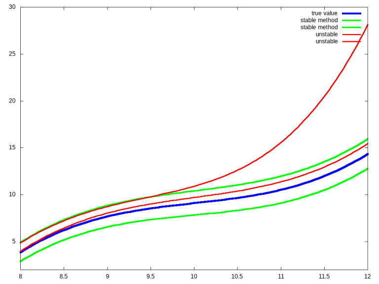
The answer lies in a property of numerical algorithm call stability. Stability means that an algorithm does not magnify errors (approximations) in the input data; instead, the error in the output can be bounded by some factor. The figure below shows a simplified example:

A stable algorithm will produce a bounded error even when starting with approximated input, whereas an unstable method will produce a small output error only for very small input errors.

The particular homegrown variant of Gaussian elimination they had attempted to implement avoided division on the left-hand side, keeping all coefficients in integers, which meant that the coefficients could grow large. On the right hand side, this led to an explosive growth in cancellation which increased the relative error in the input manifold. It was particularly perplexing to them because they had used integers intentionally in an attempt to produce a better, more numerically stable solution.

Naturally, the question then arose: how could the problem setters be confident that the problem they posed could be solved with standard methods in a numerically stable fashion?

In the course of the discussion, several points of view came to light. Some contestants believed that there's a "95% percent chance" that Gaussian elimination is unstable for at least one problem input, some believed that the risk of instability had increased because the problem required a transform into the log domain and back, some believed that Gaussian problems shouldn't be posed if they involve more than 50 variables, and some contestants thought that Gaussian elimination with partial pivoting was a "randomly" chosen method.

In short, there was a great deal of fear and uncertainty.

Here are a few facts regarding Gaussian elimination with partial pivoting contestants should know:

• Gaussian elimination (with partial pivoting) is almost always stable in practice, according to standard textbooks. For instance, Trefethen and Bau write:
  (...) Gaussian elimination with partial pivoting is utterly stable in practice. (...) In fifty years of computing, no matrix problems that excite an explosive instability are known to have arisen under natural circumstances.
  Another textbook, Golub and van Loan, write: (...) the consensus is that serious element growth in Gaussian elimination with partial pivoting is extremely rare. (begin emphasis) The method can be used with confidence. (end emphasis)