Hi everyone!
Let's continue with learning continued fractions. We began with studying the case of finite continued fractions and now it's time to work a bit with an infinite case. It turns out that while rational numbers have unique representation as a finite continued fraction, any irrational number has unique representation as an infinite continued fraction.
Part 1: Introduction
Part 2: Properties and interpretation
Distance between convergents. In the first part we learned that for continued fraction $$$r=[a_0, a_1, \dots, a_n]$$$ elements of the sequence $$$r_0, r_1, \dots, r_n$$$ where $$$r_k = [a_0, a_1, \dots, a_k]$$$ are called convergents. We also derived that subsequent convergents obey a simple formula:
Subsequent convergents seemingly should be closer to $$$r$$$ with bigger $$$k$$$, culminating in $$$r_n=r$$$. So, let's find some bound on how far away from $$$r$$$ can $$$r_k$$$ be. We may start with looking on the difference between $$$r_k$$$ and $$$r_{k-1}$$$:
Let's rewrite the numerator of this fraction:
Which means that numerator of $$$r_k - r_{k-1}$$$ is the opposite of numerator of $$$r_{k-1} - r_{k-2}$$$. The base case here is defined by $$$p_0 q_{-1} - p_{-1} q_0$$$, which is equal to $$$-1$$$. In this way we may conclude that $$$p_k q_{k-1} - p_{k-1} q_k = (-1)^{k-1}$$$, thus the whole difference is written as follows:
Further we will also need to know the distance between $$$r_{k+1}$$$ and $$$r_{k-1}$$$:
Approximation properties. Formulas above allow us to represent number $$$r=r_n$$$ as explicit telescopic sum (given that $$$r_0=a_0$$$):
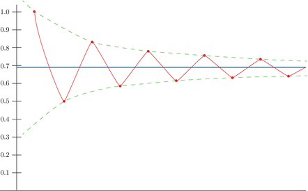
Since $$$q_k$$$ monotonically increases, we may say that $$$q_{k+1} q_k > q_k q_{k-1}$$$, thus we have an alternating sum which terms are decreasing by absolute value. This fact automatically implies several important properties, which may be illustrated by the picture below:

In our specific case difference between subsequent convergents quickly drops:
Consequent convergents maintain lower and upper bound on possible values of $$$r$$$ and each summand makes one of bounds more accurate. Bound above means that segment of possible $$$r$$$ is at least halved on each step. Few important corollaries follow from this:
- Convergents with even indices are lower than $$$r$$$ while convergents with odd indices are greater than $$$r$$$,
- If indices $$$j$$$ and $$$i$$$ have different parity then:
- If indices $$$j$$$ and $$$i$$$ have same parity and $$$j>i$$$ then:
- If $$$j>i$$$, then $$$|r_i - r| \geq |r_j - r|$$$.
These observations provide us convenient means of estimating how close is $$$r_k$$$ to $$$r$$$:
So, the final "pretty" bounds on the distance between $$$r_k$$$ and $$$r$$$ may be written as follows:
Infinite fractions. Now that we had a proper introduction of finite continued fractions, we may introduce infinite fractions $$$[a_0, a_1, a_2, \dots]$$$ as well. We say that $$$r$$$ is represented by such infinite fraction if it's the limit of its convergents:
Properties above guarantee that this series is convergent, and there is an algorithm to calculate subsequent $$$a_k$$$, which altogether means that there is one-to-one correspondence between irrational numbers and infinite continued fractions. Some well-known constants, like golden ration, have "pretty" continued fraction representations:
It is also worth noting that continued fraction is periodic if and only if $$$r$$$ is quadratic irrational, that is $$$r$$$ is the solution of some quadratic algebraic equation. In terms of convergence infinite fractions also hold most of properties of finite fractions.
Geometric interpretation. Consider sequence $$$s_k = (q_k;p_k)$$$ on 2-dimensional space. Each point $$$s_k$$$ corresponds to convergent $$$\frac{p_k}{q_k}$$$ which is the slope coefficient of the vector from $$$(0;0)$$$ to $$$(q_k;p_k)$$$. As was mentioned earlier, convergent coefficients are determined by formula:
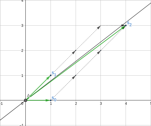
Geometrically it means that $$$s_k=a_k s_{k-1} + s_{k-2}$$$. Let's recall how coefficients $$$a_k$$$ are obtained. Let $$$b_0, b_1, \dots, b_n$$$ be the states of $$$r$$$ at each step. Thus, we initially have $$$b_0=r$$$ and then for each $$$b_k$$$ we calculate $$$a_k = \lfloor b_k \rfloor$$$ and say that $$$b_{k+1} = \frac{1}{b_k - a_k}$$$. So, for example:
If you look closely, you may see that the numerator of $$$b_k$$$ is the denominator of $$$b_{k-1}$$$ and the denominator of $$$b_k$$$ is given by:
Thus, the whole number $$$b_k$$$ may be defined as follows:
The meaning of this coefficient is as follows: Consider line $$$y=rx$$$. As convergents approach $$$r$$$, slope coefficient of $$$(q_k; p_k)$$$ approaches $$$r$$$ as well and thus points $$$(q_k; p_k)$$$ lie closer and closer to this line. That being said, value $$$|p_k - r q_k|$$$ tells us how far is $$$(q_k; p_k)$$$ from $$$y=rx$$$ on the vertical line $$$x=q_k$$$. Note that $$$s_{k-1}$$$ and $$$s_{k-2}$$$ are always on opposite sides from line $$$y=rx$$$, so adding $$$s_{k-1}$$$ to $$$s_{k-2}$$$ will decrease vertical distance of $$$s_{k-2}$$$ by $$$|p_{k-1} - r q_{k-1}|$$$. In this way we can see that $$$a_k = \lfloor b_k \rfloor$$$ is nothing but the maximum amount of times we may add $$$s_{k-1}$$$ to $$$s_{k-2}$$$ without switching the sign of $$$p_{k-2} - r q_{k-2}$$$. This gives geometric meaning to $$$a_k$$$ and the algorithm of computing them:

Algorithm above was taught to Vladimir Arnold by Boris Delaunay who called it "the nose stretching algorithm". This algorithm was initially used to find all lattice points below the line $$$y=rx$$$ but also turned out to provide simple geometric interpretation of continued fractions.
This connection between continued fractions and 2d-geometry established the notion of mediants. That is, for fractions $$$A = \frac{a}{b}$$$ and $$$B = \frac{c}{d}$$$ their mediant is $$$C = \frac{a+c}{b+d}$$$. If $$$A$$$ and $$$B$$$ are slope coefficients of two vectors, then $$$C$$$ is the slope coefficient of the sum of these vectors.
That should be all for now, next time I hope to write in more details about how the nose stretching algorithm may be used to count lattice points under the given line without that much pain and to solve integer linear programming in 2D case. Also I'm going to write about how continued fractions provide best rational approximations and, hopefully, write more about competitive programming problems where this all may be used, so stay tuned!


