Hello Codeforces,

Before we start: Thanks to bashkort for hosting this year's Codeforces Month of Blog Posts Challenge and giving me some motivation to actually finish this blog.

This is the second blog on the series about the applications of the rotating calipers technique. If you haven't read the first part yet, make sure to check it out, as much of the terminology that was introduced throughout the first part is going to be used here without further explanation. In this blog, a few more advanced applications will be presented.

Short recap of the main terminology

• Line of support: a line $$$l$$$ that intersects the boundary of the polygon such that the entire polygon lays on one side of $$$l$$$
• Anti-podal pair: a pair of vertices which have two parallel lines of support intersecting them
• Rotating calipers: an algorithm where parallel lines of support get rotated around the polygon while being kept on the boundary of the polygon at all times

Minimum-area enclosing rectangle of a convex polygon

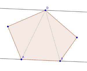
The first application that is going to be discussed is the minimum area enclosing rectangle problem. For a given polygon $$$P$$$, the problem asks us to find a minimum area rectangle $$$R$$$ such that all points of the polygon are inside that rectangle. It is quite clear why all 4 sides of the rectangle must lay on the boundary of $$$P$$$. However, an even stronger result can be obtained: If the area is minimum, then one of the sides of the rectangle has to intersect an edge of the polygon. To understand why, consider the contrary scenario: each side of the rectangle $$$R$$$ intersects with exactly one vertex of $$$P$$$, and the area of $$$R$$$ is still minimum possible. Let's call these vertices $$$p_a$$$, $$$p_b$$$, $$$p_c$$$, $$$p_d$$$, in clockwise order. $$$R$$$ has side lengths $$$l_1$$$ and $$$l_2$$$ respectively. An example of what this can look like:

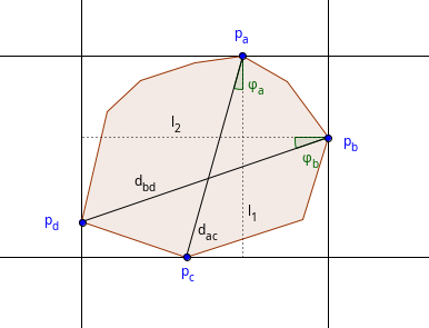
The area of the rectangle is $$$A = l_1 \times l_2$$$. Rotating the rectangle by a small angle $$$ \theta $$$ changes the side lengths of the rectangle. What happens usually is that there exists a direction of rotation where $$$l_1$$$ increases, and another direction where $$$l_1$$$ decreases. There are two possible scenarios of what might happen:

1. There exists a direction of rotation which allows both $$$l_1$$$ and $$$l_2$$$ to be decreased.
2. One direction of rotation would increase $$$l_1$$$ and would decrease $$$l_2$$$, and vice versa.

In the first case, it is clear that a rotation would result in a lower total area. However, for the second case, it isn't as clear why it is possible to get a smaller area. So, without loss of generality we will assume that $$$\varphi_{a} > \varphi_{b}$$$ and we rotate the polygon by $$$\theta$$$ degrees. The following also holds true:

Rotating by $$$\theta$$$ degrees would change last equation into:

To see why $$$A' < A$$$, we have to take a look at the cosine function for values between $$$0$$$ and $$$ \frac{\pi}{2}$$$:

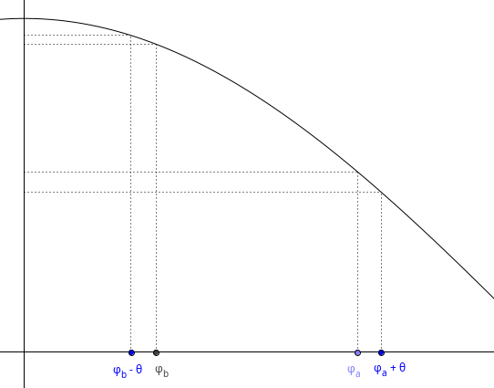
We can see that $$$cos(\varphi_a + \theta )$$$ got closer to 0 than $$$cos(\varphi_b -\theta )$$$ got to 1. Therefore, the total area must have gotten smaller.

Now that we know that each minimum area enclosing rectangle touches at least one of the edges of the polygon, we can now use the rotating calipers technique to solve this problem. The only difference between the standard rotating calipers technique and this variation is that we maintain 4 lines instead of just two, and these 4 lines together must form an enclosing rectangle. Essentially, we are maintaining a "rotating rectangle" around the polygon. One of the main difficulties of the implementation would be the criteria on when to stop rotating because a $$$90^{\circ}$$$ degree has been reached. For that, we'll make use of the dot product. Take a look at the following image:

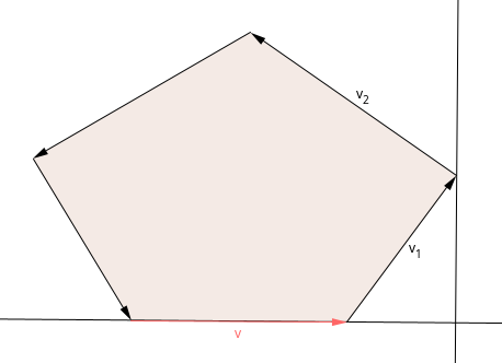
The following two properties hold true:

So, whenever there occurs a sign change in the dot product, we know that we can stop rotating further. The total runtime of this algorithm would be $$$O(4*n) \in O(n)$$$, since the enclosing rectangle contains 4 edges and maintaining them takes $$$O(n)$$$ steps each.

Minimum-perimeter enclosing rectangle

The minimum perimeter enclosing rectangle problem is very similar to the minimum-area version. Just as in the previous section, if the perimeter is minimum then at least one of the edges of $$$P$$$ must intersect with an edge of the rectangle. To see why this is the case, consider the opposite scenario. Define $$$p_i (1 \leq i \leq 4)$$$ to be the vertices that intersect with the rectangle. Also, define angles $$$\alpha_i$$$ and $$$\beta_i$$$ like this:

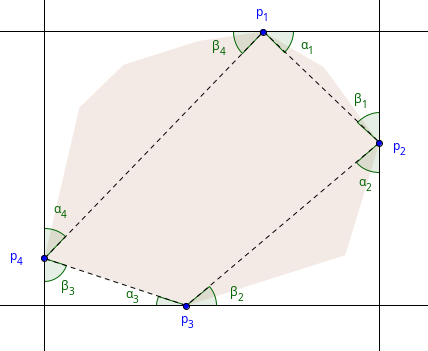
From the law of sines, we can conclude that the perimeter $$$p_m$$$ must be:

Let $$$\theta_{min} < 0 < \theta_{max}$$$ be the angles of rotation which make one of the edges of $$$P$$$ intersect with the rectangle. We can now reformulate the perimeter $$$p_m$$$ as a function with a variable $$$\theta \in [ \theta_{min}, \theta_{max} ]$$$, which represents the perimeter after we rotate the polygon by $$$\theta$$$ degrees:

Since $$$\alpha_i + \theta$$$ and $$$\beta_i - \theta$$$ are angles of a triangle, $$$|(\alpha_i + \theta) - (\beta_i - \theta)| \leq \frac{\pi}{2} $$$ must hold true. Each of the summands of $$$p_m(\theta)$$$ describe a concave function, since $$$cos(x)$$$ for $$$-\frac{\pi}{2} \leq x \leq \frac{\pi}{2}$$$ is concave. The sum of concave functions describe a concave function as well, so $$$p_m(\theta)$$$ must be a concave function. One nice property about concave functions is that the minimum value of the function is determined by the "edge" values for $$$\theta$$$, in our case by either $$$\theta_{min}$$$ or by $$$\theta_{max}$$$. This would mean that we can rotate the polygon by either $$$\theta_{min}$$$ or $$$\theta_{max}$$$ degrees to make the perimeter smaller. By that rotation, we manage to make one edge of the polygon intersect with the rectangle.

Now that we know that the minimum-perimeter rectangle has at least one of the sides collinear with the polygon, we can apply more or less the same algorithm as above, but instead of calculating the minimum total area we calculate the minimum total perimeter.

Merge two convex hulls

Merging two convex hulls into one convex hull can be done with a simple convex hull implementation. However, this is somewhat of an overkill, since we nearly don't have to do as many calculations with the rotating calipers technique as we would need to do with a regular convex hull implementation. To understand why using a convex hull algorithm would be an overkill here, let's take a look at an example:

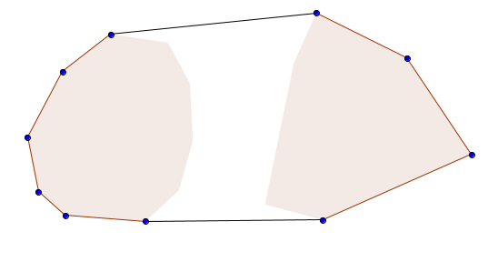
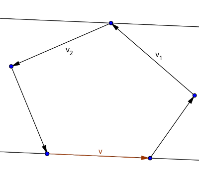
As we can see, to merge two convex hulls into one, we only need to find the two new edges that connect the two hulls and delete the vertices inside the interior. The edges that we need to find are called bridges. From the image above, we can see that the bridges, if extended, would form lines of support for both polygons $$$P$$$ and $$$Q$$$. So, in short, we need to find all lines of support that are lines of support for both polygons, and they must be lines of support in the same direction. A co-podal pair is a pair of vertices of $$$P$$$ and $$$Q$$$ that admit parallel lines of support in the same direction. So unlike with anti-podal pairs, which lay on opposite sides of the polygons, co-podal pairs must lay on the same side of the polygons respectively.

Consider a co-podal pair $$$p_i \in P$$$, $$$q_k \in Q$$$. The line $$$L = (p_i, q_k)$$$ is a bridge if and only if all vertices $$$p_{i-1}$$$, $$$p_{i+1}$$$, $$$q_{k-1}$$$ and $$$q_{k+1}$$$ lay on the same side of $$$L$$$. That holds true because if all of these vertices lay on the same side of $$$L$$$, then the line between $$$p_i$$$ and $$$q_k$$$ must be a line of support for both $$$P$$$ and $$$Q$$$. A simple algorithm description would be to generate all possible co-podal pairs and then check whether the 4 vertices mentioned above lay on the same side of the line between the co-podal pair. Note that this algorithm also works for intersecting polygons, a little bit of extra work has to be done however if one polygon is contained within the other. Also note that in certain cases, you need 4 bridges instead of two:

Critical support lines

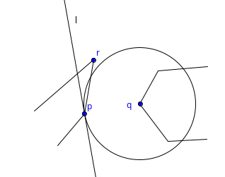
Critical support (in short "CS") lines are lines of support of two polygons $$$P$$$ and $$$Q$$$ such that the polygons lay on opposite sides of the line. This line acts as a separating line between the two polygons. An image to visualize what we're trying to find here:

This problem is indeed very similar to the previous problem. Let $$$L = (p_i, q_k)$$$ with $$$p_i \in P, q_k \in Q$$$ be a CS line. The pair $$$(p_i, q_k)$$$ must be an anti-podal pair, since they admit the same line of support $$$L$$$, and they lay on opposite sides of the polygons. Also, the vertices $$$p_{i-1}$$$ and $$$p_{i+1}$$$ are not allowed to lay on the same side of $$$L$$$ as $$$q_{k-1}$$$ and $$$q_{k+1}$$$. Turns out, these two conditions are enough to determine whether a line is a CS-line or not.

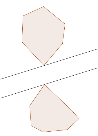
Maximum width separating strip between two convex polygons

In this problem, we want to find the maximum width of a separating strip between two non-intersecting convex polygons $$$P$$$ and $$$Q$$$. A separating strip is defined by two parallel lines, one of which is a line of support for $$$P$$$, and the other is for $$$Q$$$. Between these two lines, there isn't allowed to be a vertex of neither $$$P$$$ nor $$$Q$$$:

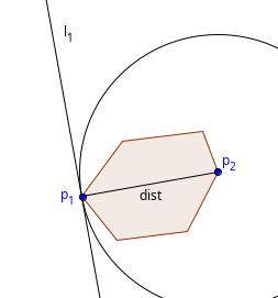
This is one example where we can use CS lines. If a vertex lays on the boundary of the separating strip, then it must be a vertex in between the two CS lines. Let the vertices $$$p_i \in P, q_k \in Q$$$ be the vertices that lay on the boundary of the separating strip. The pair $$$(p_i, q_k)$$$ must be an anti-podal pair. There are two possible cases that need to be considered:

1. The line between $$$p_i$$$ and $$$q_k$$$ intersects one edge of either $$$P$$$ or $$$Q$$$. For that case, the rotating calipers algorithm is going to be used, iterating over every edge of $$$P$$$ and $$$Q$$$ and checking every anti-podal pair (a pair here denotes a pair of an edge and a vertex, not a pair of two vertices).
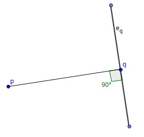
2. The line between $$$p_i$$$ and $$$q_k$$$ doesn't intersect any edge. In that case, the width of the strip is going to be defined as the distance between the two vertices. However, we need an additional criterion to check whether such a pair even allows a strip with that width. Consider the line $$$L(p_i, q_k)$$$. A sufficient criterion would be if the angle between $$$L$$$ and each one of the edges $$$(p_{i-1}, p_i), (p_i, p_{i+1}), (q_{k-1}, q_k), (q_k, q_{k+1})$$$ to be greater that $$$90^{\circ}$$$.

Since there exist $$$O(n+m)$$$ anti-podal pairs for both cases, the total runtime of the algorithm would be, again, $$$O(n+m)$$$.

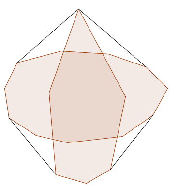
Minkowski sums of two convex polygons

In the last section of this blog, we will discover how to calculate the minkowski sums of two convex polygons using the rotating calipers technique. There exist other methods for achieving the same (such as sorting the edges by their polar angles) with the same time complexity, but this series wouldn't be complete without at least mentioning this application. So, what is the minkowski sum? The minkowski sum of two polygons $$$P$$$ and $$$Q$$$ is simply a new polygon that contains every possible sum of two points $$$p \in P$$$ and $$$q \in Q$$$. Formally, you can define the minkowski sum as:

while $$$p+q$$$ represents a vector addition. The first thing that we're going to look at is the fact that $$$P \oplus Q$$$ is a convex polygon as well. To see why this is true, we have to show that for every pair of points $$$pt_1, pt_2 \in P \oplus Q$$$, every point on the segment between $$$pt_1$$$ and $$$pt_2$$$ lays inside the minkowski sum as well. This segment can be described as:

Decompose $$$pt_1$$$ and $$$pt_2$$$ into their original vectors from $$$P$$$ and $$$Q$$$:

Now rewrite the line segment equation as:

The first summand must be a point between $$$p_1$$$ and $$$p_2$$$, and since $$$P$$$ is convex, it must lay inside $$$P$$$. Similarly, the second summand must lay inside $$$Q$$$. In total, this means that any point between $$$pt_1$$$ and $$$pt_2$$$ must lay inside the minkowski sum, therefore, the minkowski sum must be a convex polygon.

Now, what would you do if you wanted to construct the leftmost vertex of the minkowski sum? Since the $$$x$$$-value of the vertex would have to be minimum possible, it would only make sense to take the leftmost vertex of both $$$P$$$ and $$$Q$$$, since these vertices $$$x$$$-value is the smallest it could get. The same line of argument can be used if we want to compute the rightmost / highest / lowest vertex of the minkowski sum. Turns out, this argument can be generalized not for just only these 4 directions, but to all possible directions. So, if we want to have the diagonally left bottommost vertex of the sum, it only makes sense to take the diagonally left bottommost vertex of both polygons and sum them up etc. Such vertices are called extreme points for a specific direction. One nice property about these extreme points is that they form co-podal pairs. This holds true because parallel lines of support essentially have the same direction.

Since every vertex of the minkowski sum is also an extreme point for a specific direction, all vertices of that polygon must be sums of co-podal pairs of $$$P$$$ and $$$Q$$$. We can now use the rotating calipers algorithm to calculate the minkowski sum $$$P$$$ and $$$Q$$$.

The algorithm

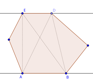
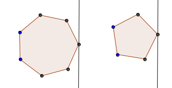
First, we will calculate the point with the minimum $$$y$$$-coordinate and set that as our starting point. We then set up two horizontal lines that will act as parallel lines of support throughout this algorithm. This might look like this:

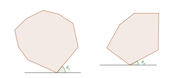
First, add the point with the minimum $$$y$$$-coordinate to our set of vertices. Then, while rotating around the polygon, we need to take care of a few cases. Assume that the sum $$$p_i + q_j$$$ was the last vertex that was added to the set of vertices:

1. $$$\theta_p < \theta_q$$$: rotate by $$$\theta_p$$$ degrees and add $$$p_{i+1} + q_j$$$ to the set of vertices.
2. $$$\theta_p > \theta_q$$$: rotate by $$$\theta_q$$$ degrees and add $$$p_i + q_{j+1}$$$ to the set of vertices.
3. $$$\theta_p = \theta_q$$$: rotate by $$$\theta_p$$$ degrees and add $$$p_{i+1} + q_{j+1}$$$ to the set of vertices.

And that's it! The total runtime of this algorithm is $$$O(n+m)$$$, which is in fact optimal, since the minkowski sum has up to $$$n+m$$$ vertices.

Conclusion

Here, a few more applications of the paradigm were discussed. The huge number of problems that can be tackled using such a simple paradigm is the reason why I think that the rotating calipers is such an amazing algorithm. Hopefully, I was able to convince you of the same. If you have any questions about this blog, please let me know in the comments. There exist more applications of the algorithm, but I decided not to include them in this blog since they are too complex for a CP setting.

Hello Codeforces,

this blog is going to be about the rotating calipers technique. Apparently, it's a basic technique that can be used to solve various problems on convex polygons, however, I couldn't find a codeforces blog about it, so I just decided to write one.

General idea behind the algorithm

For the following, we are going to assume that $$$P$$$ is a convex polygon in the 2D plane with a non-negative area. Furthermore, we are going to assume that no three points of the polygon are collinear, meaning that the angle at each vertex of the polygon is smaller than $$$180^{\circ}$$$. We call a line $$$l$$$ a line of support if it intersects the boundary of the polygon, but not its interior. Suppose that we have two parallel lines of support, $$$l_1$$$ and $$$l_2$$$. It is pretty straightforward that both of these lines lay on opposite sides of the polygon respectively. You could for example set the line $$$l_1$$$ to a vertical line intersecting the leftmost vertex, and $$$l_2$$$ intersecting the rightmost one. Rotating the two lines around the polygon, while they are kept tightly on its border is the fundamental idea of the rotating calipers technique. Here's an animation of what this might look like:

Additionally, a pair of vertices $$$(v_1, v_2), v_1, v_2 \in P$$$ is called an anti-podal pair if there exist two parallel lines of support that intersect with the vertices $$$v_1$$$ and $$$v_2$$$ respectively.

Finding the diameter of a convex polygon

The first application of the rotating calipers technique that is going to be considered is the calculation of the diameter of a convex polygon, or the largest distance between two points that lay inside the polygon in $$$O(n)$$$ time. Note that if the polygon is not convex, then you can simply calculate the convex hull of the polygon and then apply the following algorithm.

Let $$$p_1$$$ and $$$p_2$$$ be the points that define the diameter of the polygon, e.g. $$$dist(p_1, p_2)$$$ is the maximum possible distance inside the polygon. It is not difficult to see that $$$p_1$$$ and $$$p_2$$$ must lay on the boundary of the polygon, simply because if you draw a line from $$$p_1$$$ to $$$p_2$$$, you're able to extend that line to the boundary, and that way you have found a greater distance. Actually, the two points that define the diameter must be vertices of the polygon. Why? Assume that $$$p_1$$$ lays on an edge of the polygon. Then, there are two directions you could move $$$p_1$$$ to. One of them increases the distance to $$$p_2$$$ and one of them decreases it. Choose the direction that increases the distance and move the point to that direction. This contradicts the assumption that $$$dist(p_1, p_2)$$$ is maximum possible, so the point $$$p_1$$$ cannot lay on the edge of the polygon. We can even prove a stronger result: $$$(p_1, p_2)$$$ is an anti-podal pair!

Construct a circle $$$C$$$ with a center at $$$p_2$$$ and a radius of $$$dist(p_1, p_2)$$$. The points of the polygon must all lay inside the circle, because otherwise $$$p_1$$$ and $$$p_2$$$ wouldn't have the maximum possible distance. Now construct a tangent line $$$l_1$$$ at the point $$$p_1$$$. By definition, the tangent line doesn't intersect the interior of the circle, so it also doesn't intersect the interior of the polygon. Therefore, $$$l_1$$$ has to be a line of support. Now repeat the same procedure with a circle centered around $$$p_1$$$, and the resulting line of support is called $$$l_2$$$. It is easy to see that $$$l_1$$$ and $$$l_2$$$ are parallel to each other. Altogether, the pair $$$(p_1, p_2)$$$ must be an anti-podal pair:

Now that we know that $$$(p_1, p_2)$$$ is an anti-podal pair, we could construct a simple algorithm for calculating the diameter:

1. Calculate all possible anti-podal pairs
2. Return the maximum possible distance of all anti-podal pairs

However, there are two open questions remaining:

1. If we want the algorithm to be efficient, we need to know how many anti-podal pairs there are
2. How can we calculate all possible anti-podal pairs efficiently?

Upper bound on the number anti-podal pairs

Consider any anti-podal pair $$$(p_1, p_2)$$$ (the distance between them doesn't have to be the diameter, it just has to be an anti-podal pair). By definition, there have to be two parallel lines of support $$$l_1, l_2$$$ that intersect the vertices $$$p_1$$$ and $$$p_2$$$ respectively. Now, we can rotate these parallel lines simultaneously until they hit an edge of the polygon. That way, it is possible to map every anti-podal pair to a pair of either two edges or an edge and a vertex. In an algorithm that calculates all anti-podal pairs, it would be sufficient to check for every edge its parallel line of support.

Now there are two cases that need to be considered:

Case 1: The parallel line of support only intersects a vertex. From the image below, we can conclude that there are two anti-podal pairs related to edge $$$AB$$$: The pairs $$$(A, D)$$$ and $$$(B, D)$$$.

Case 2: The parallel line intersects an edge of the polygon. In the image below, we can see that there are 4 possible anti-podal pairs. Since we are looking at two edges however, we can say that each edge accounts for $$$4 / 2 = 2$$$ pairs.

So we can conclude that the number of anti-podal pairs is at most $$$2*n \in O(n)$$$, while $$$n$$$ is the number of edges/vertices of the polygon. Note that it's possible to prove tighter bounds, but for the simplicity of this blog it's enough to have proven that the number of anti-podal pairs is in $$$O(n)$$$.

Algorithm for generating all anti-podal pairs

Our algorithm now consists of iterating over every edge while maintaining a parallel line of support. That's where the rotating calipers technique is going to be used. When going from one edge to the next one, we keep rotating the line of support around the polygon until the lines are parallel again. When an edge is being visited, the anti-podal pairs can be generated the way it was described in the previous section. The algorithm somewhat resembles the two pointer technique. However, as it is with many other geometry problems, the main difficulty does not lay in the description of the solution, but rather in its correct implementation.

In this implementation, the edges are like vectors from one vertex $$$v_i$$$ to the next vertex $$$v_{i+1}$$$. The vertices of the polygon must be sorted in either clockwise or counterclockwise order, the code should work for both. The main difficulty is the criteria on when to stop rotating the parallel line. For that, we'll take a look at an example:

The following two properties hold true:

We observe that there occurs a sign change in the cross product whenever we reach the vertex that allows a parallel line of support. So whenever this occurs, we stop rotating the parallel line. The runtime of this algorithm is $$$O(n)$$$, because iterating over all edges takes $$$O(n)$$$ time, and the parallel line visits every vertex at most once. The implementation:

#define ll long long
#define pii array<int,2>
#define nx(i) (i+1)%n
#define pv(i) (i-1+n)%n

struct Point {
    ll x,y;
 
    Point operator+(const Point &p) {
        return {x + p.x, y + p.y};
    }

    Point operator-(const Point &p) {
        return {x - p.x, y - p.y};
    }
};

ll cross(Point p1, Point p2) {
    return p1.x * p2.y - p1.y * p2.x;
}

int sign(ll num) {
    if (num < 0) return -1;
    else if (num == 0) return 0;
    else return 1;
}

vector<pii> all_anti_podal(int n, vector<Point> &p) {
    int p1 = 0, p2 = 0; // two "pointers"
    vector<pii> result;

    // parallel edges should't be visited twice
    vector<bool> vis(n, false);

    for (;p1<n;p1++) {
        // the edge that we are going to consider in this iteration
        // the datatype is Point, but it acts as a vector
        Point base = p[nx(p1)] - p[p1];

        // the last condition makes sure that the cross products don't have the same sign
        while (p2 == p1 || p2 == nx(p1) || sign(cross(base, p[nx(p2)] - p[p2])) == sign(cross(base, p[p2] - p[pv(p2)]))) {
            p2 = nx(p2);
        }

        if (vis[p1]) continue;
        vis[p1] = true;

        result.push_back({p1, p2});
        result.push_back({nx(p1), p2});
        
        // if both edges from p1 and p2 are parallel to each other
        if (cross(base, p[nx(p2)] - p[p2]) == 0) {
            result.push_back({p1, nx(p2)});
            result.push_back({nx(p1), nx(p2)});
            vis[p2] = true;
        }
    }

    return result;
}

Width of a convex polygon

Now that we are able to calculate the diameter of a convex polygon, we want to see what other problems we can use the rotating calipers technique for. Let the width of a convex polygon be the shortest distance between two parallel lines of support. The width is like the minimum distance that two walls would need to have such that the entire polygon would fit in between these walls. If the polygon is not convex then we can again just calculate the convex hull and then apply the same procedure.

We can use the same algorithm that we used for the previous problem. We iterate over every edge of the polygon and maintain a parallel line of support $$$l$$$ to the edge. $$$l$$$ can either intersect with an edge or with a vertex of the polygon. Let's look at both of these cases separately:

1. $$$l$$$ intersects with a vertex. Then all you have to do is to calculate the distance from that vertex to the edge.
2. $$$l$$$ intersects with an edge. Select any point on the line $$$l$$$ and calculate the distance to the edge.

After doing all of these calculations, you return the minimum value as the final result. The algorithm has a total runtime of $$$O(n)$$$.

Minimum distance between two convex polygons

Another application for the rotating calipers technique is the problem of the minimum distance between two convex polygons. Note that here, the polygons must be convex from the beginning, unlike in previous problems, where the calculation of a convex hull was sufficient. Additionally we assume that the polygons don't intersect each other, otherwise, the minimum distance would be 0.

Let $$$P$$$ and $$$Q$$$ be two convex polygons, and we want to calculate the minimum distance between them. Let $$$p$$$ and $$$q$$$ be the points that fulfill that minimum distance, e.g. $$$p \in P$$$, $$$q \in Q$$$ and $$$dist(p, q)$$$ is minimum possible. $$$p$$$ and $$$q$$$ must lay on the boundaries of $$$P$$$ and $$$Q$$$ respectively. Furthermore, who would have guessed it, the points $$$p$$$ and $$$q$$$ admit parallel lines of support.

The aforementioned claim is not easy to see, so let's prove it. For that, we need to consider three cases:

Case 1: $$$p$$$ and $$$q$$$ are vertices. We construct a circle $$$C$$$ with $$$q$$$ as a center and $$$dist(p, q)$$$ as the radius. There are obviously no vertices of $$$P$$$ inside $$$C$$$, because that would mean that a smaller distance would be possible. Construct a tangent line $$$l_p$$$ to the circle through $$$p$$$. The claim now is that $$$l_p$$$ is a line of support. Assume that $$$l_p$$$ is not a line of support, e.g. it intersects with the interior of $$$P$$$. Here's an image of what this could look like:

The problem with the assumption becomes pretty clear: A part of the edge between $$$p$$$ and $$$r$$$ lays inside the circle, so a shorter distance than $$$dist(p, q)$$$ is possible. However, that's a contradiction and so $$$l_p$$$ must be a line of support. We can construct another line of support $$$l_q$$$ using the same line of argument. Additionally, $$$l_p$$$ and $$$l_q$$$ are parallel by definition of tangent lines.

Case 2: One point lays on a vertex and the other point on an edge. Without loss of generality, we assume that point $$$p$$$ is a vertex of $$$P$$$ and $$$q$$$ lays on an edge $$$e_q$$$ of $$$Q$$$. Construct a line of support $$$l_p$$$ similar to how it was done in case 1. Now we need to prove that $$$l_p$$$ is parallel to the edge $$$e_q$$$. This follows from the fact that the distance between $$$p$$$ and $$$q$$$ is minimum possible.

Since the distance between $$$p$$$ and $$$q$$$ is minimum possible, the angle in the image above must be exactly $$$90^{\circ}$$$. The angle between $$$l_p$$$ and the line between $$$p$$$ and $$$q$$$ must be $$$90^{\circ}$$$ as well, therefore, $$$l_p$$$ and the edge $$$e_q$$$ are parallel to each other.

Case 3: Both $$$p$$$ and $$$q$$$ lay on an edge. These edges must be parallel to each other, because if they wouldn't, then we could find a shorter distance where either case 1 or case 2 applies. So, $$$p$$$ and $$$q$$$ also admit parallel lines of support, namely the lines that go through the edges.

The algorithm for minimum distance between two polygons

Now that we know that $$$p$$$ and $$$q$$$ admit parallel lines of support, the rotating calipers algorithm comes back into play. But instead of having two calipers for each polygon, we now have only one caliper per polygon. However, we must pay attention on how we place these calipers initially. If we were to set the calipers like this for example:

then we could never reach $$$p$$$ and $$$q$$$ at the same time. One way to solve this problem is to initially set the caliper for polygon $$$P$$$ to be a vertical line intersecting with the leftmost vertex of $$$P$$$. Similarly, the caliper for polygon $$$Q$$$ is a vertical line intersecting with the rightmost vertex of $$$Q$$$. As we did for calculating the diameter, we iterate over every edge of $$$P$$$. Let $$$(p_i, p_{i+1})$$$ be the edge of $$$P$$$ that we are currently visiting. Furthermore, let $$$q_j$$$ be the vertex of $$$Q$$$ that is currently visited. We now have to check for all three cases that were mentioned in the last proof:

1. Vertex-vertex case: check $$$dist(p_i, q_j)$$$ and $$$dist(p_{i+1}, q_j)$$$ and update the minimum value accordingly.
2. Edge-vertex case: check the distance between the line segment $$$(p_i, p_{i+1})$$$ and $$$q_j$$$ and update the minimum value accordingly.
3. Edge-edge case: check the distance between the line segments $$$(p_i, p_{i+1})$$$ and $$$(q_j, q_{j+1})$$$. However, this is only possible if these line segments are parallel to each other.

To complete the calculation, you'd have to iterate over all edges of $$$Q$$$ as well. The runtime of this algorithm is $$$O(n+m)$$$, while $$$n = |P|, m = |Q|$$$.

Maximum distance between two polygons

The algorithm for calculating the minimum distance can be perfectly translated to calculating the maximum distance. The only change one would have to make is to take the maximum over all possible calculated values instead of the minimum. Literally. That's all you have to do. Unlike in the previous problem, the algorithm should also work for intersecting polygons. The proof of correctness also becomes much easier:

Let $$$p$$$ and $$$q$$$ be the points in $$$P$$$ and $$$Q$$$ respectively with maximum distance. $$$p$$$ and $$$q$$$ admit parallel lines of support. Construct a circle $$$C_q$$$ with center $$$q$$$ and diameter $$$dist(p, q)$$$. Then, construct a line $$$l_p$$$ through point $$$p$$$ tangent to $$$C_q$$$. $$$l_p$$$ must be a line of support, since all vertices of $$$P$$$ have to lay inside $$$C_q$$$, otherwise, a greater distance would be achievable. Construct $$$l_q$$$ analogously. By definition of tangent lines, $$$l_p$$$ and $$$l_q$$$ must be parallel.

Note that calculating the hull of both polygons together and then running the diameter algorithm from above does not always work, because the diameter of $$$P$$$ might be larger than the greatest distance between polygons $$$P$$$ and $$$Q$$$.

Conclusion

In this blog, a few basic applications of the rotating calipers technique were discussed. Those are by all means not all applications that exist out there, but rather a few basic ones to understand in which ways we can apply this technique. A few problem links:

• Robert Hood
• Problem K — Trash Removal
• Bridge Across Islands
• Fence Orthogonality

Currently, I'm working on my own problemset about rotating calipers, click on this link if you want to check it out.

UPD: Part 2 of this blog is out

Hello,

so this article on USACO Guide explains an alternative way to implement a solution for the Manhattan MST problem, which is to run a modified Dijkstra algorithm that stores the distance to a node of the MST for each square of the grid. It starts at an arbitrary point in the input, and this point has a distance of zero to the MST. Then, a modified Dijkstra is run, with the difference being that whenever we encounter a square which is inside the input, we reset the distance of the square to the MST to zero.

However, this modified version of Dijkstra is not really the same as Dijkstra, because if a square is found that is part of the input, the distance to the MST gets reset to zero, and therefore, its neighboring squares get visited multiple times etc. Therefore, it's not possible to claim that this algorithm has the same running time as Dijkstra, because in Dijkstra, every node gets visited exactly once. However, the maximum number of times that a square can get visited is apparently 4 (I stress-tested the algorithm and that was the maximum number that I found). Could anyone explain the reasoning behind the 4 being the "magic upper bound" for the number of times that a square gets visited? Or could someone maybe prove me wrong and provide a sample where we visit some square at least five times?

Hello,

could anyone please explain me the intuition behind the solution of CSES-Network Renovation?

Why does this greedy strategy suffice for connecting the entire tree?

Hello Codeforces community,

could anyone recommend me any LIS related tasks that I can use to practice this topic? I find it quite difficult to find any tasks who's main solution is something regarding LIS.

Here are the tasks that I found until now:

Consecutive Subsequence

Towers (CSES)

Korney Korneevich and XOR (easy version)

Increasing Subsequence(CSES)

Copil Copac Draws Trees

Candy (BOI 2009)

Thanks in advance