This blog was going to be translation of $$$[1]$$$ (which is in Chinese) but I think I ended up deviating too much from the source material that it would not be appropriate to call this a translation. Anyways, I am honestly amazed by how ahead of its time this paper is. In its abstract, it starts by saying that the state of art for tree path queries is $$$O(n \log n + q \sqrt n \log n)$$$, which I honestly can't fathom how one would arrive, then proceeds to claim that it has found an $$$O((n+q) \log n)$$$ algorithm. All the more, in 2007.
While I was in the process of writing this blog, smax sniped me and posted $$$[9]$$$. However, we will focus on static trees only.
Thanks to oolimry, Everule and timreizin for proofreading.
Note to reader: I am expecting the reader to be familiar with what a splay tree and HLD is. You do not really need to know why splay trees are $$$O(\log n)$$$ amortised but you should know what the zig, zig-zig and zig-zag operations are. Also, when I say some algorithm has some complexity, I usually mean that it has that complexity amortised. You can probably tell from context which ones are amortised complexity. Also, there is basically $$$0$$$ reason to use the techniques described in this blog in practice (except maybe in interactive problems?), the constant factor is too high. You can scroll to the bottom to see the benchmarks. Then again, my implementation of normal HLD uses a really fast segment tree and my implementation $$$O((n+q) \log n)$$$ algorithm might have a really big constant factor.
Splay Trees
First, we want to talk about splay trees $$$[2]$$$, specifically why splay trees have amortised $$$O(\log n)$$$ complexity for splaying some vertex $$$v$$$.
Define:
- $$$s(v)$$$ as the size of the subtree of $$$v$$$
- $$$r(v)=\log s(v)$$$, the rank function
There are $$$3$$$ types of operations we can perform on a vertex when we are splaying it to the root — zig, zig-zig, zig-zag. Let $$$r$$$ and $$$r'$$$ be the rank functions before and after we perform the operation. The main results we want to show is that:
- zig has a time complexity of $$$O(r'(x)-r(x)+1)$$$ amortised
- zig-zig and zig-zag has a time complexity of $$$O(r'(x)-r(x))$$$ amortised
I will not prove these as you can find the proof in $$$[2]$$$. But the point is that through some black magic, the only operation that has a cost with a constant term is a zig operation, which we only perform once. Somehow, we manage to remove all constant terms from our zig-zig and zig-zag operations.
Let $$$r_i$$$ be the rank function after performing the $$$i$$$-th operation. Suppose that we have performed $$$k$$$ operations on to splay some vertex, then the total time complexity is $$$O((r_{k}(x)-r_{k-1}(x))+(r_{k-1}(x)-r_{k-2}(x))+\ldots+(r_{1}(x)-r_{0}(x))+1)=O(r_k(x)-r_0(x)+1)$$$. The black magic from removing all constant terms from our zig-zig and zig-zag operation is that no matter how many zig-zig and zig-zag operations we perform, they don't have any effect on the final complexity since we cancel out all the terms in a telescoping sum manner (which also explains why performing zigs only would make the complexity blow up, as we should expect). For the case of splay trees, $$$r_k(x)=\log n$$$, since $$$x$$$ becomes the root of the tree, so we obtain the complexity of $$$O(\log n)$$$.
Link-Cut Trees
Now, let's discuss why link cut trees $$$[3]$$$ have a complexity of $$$O(\log n)$$$. Here is an image of link cut trees from $$$[4]$$$.
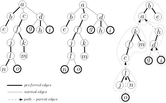
We split the tree into disjoint chains. Internally, each chain is a splay tree storing elements in the order of depth (lowest depth to the left and highest depth to the right). This way, when we splay $$$x$$$ in its splay tree, the vertices to its left are those with lower depth and the vertices to its right are those with higher depth. $$$2$$$ disjoint chains which are connected by an edge in the original tree would be connected by a path-parent edge in the new tree. If chains $$$a$$$ and $$$b$$$ were connected, with $$$a$$$ being the parent of $$$b$$$, then there would be a path-parent edge from the root of the splay tree containing $$$b$$$ to $$$a$$$. That is for each splay tree, only its root will have a path-parent edge. In the image, the tree on the left is the initial tree which is stored internally by the structure of splay trees on the right. It is good to mention now that we can actually view these disjoint splay trees as a single giant splay tree by not caring about which edge types join the vertices internally (and not caring about the fact that vertices can only have at most 2 children).
An important operation on link-cut trees is the $$$access(x)$$$ operation, which given some $$$x$$$ that we have chosen, changes the chains in such a way that the chain containing the root of the original tree also contains the vertex $$$x$$$. This is done by repeatedly ascending into the highest vertex in each chain, and switching which child is connected to its parent. So the cost of this operation is related to the number of distinct chains on the path from $$$x$$$ to the root of the whole tree. Also, we will shorten the chain of $$$x$$$ to have the deepest vertex be $$$x$$$ for reasons that will be apparent later. In the above image, we have performed $$$access(l)$$$ to get the state being the middle tree.
In pseudo-code, the access function would look something like this:
1. access(x):
2.     splay(x)
3.     if (right(x)!=NULL):                  //disconnect the current child
4.         path_parent(right(x))=x
5.         right(x)=NULL
6.     while (path_parent(x)!=NULL):        //it is now the root
7.         par=path_parent(x)
8.         splay(par)
9.         if (right(par)!=NULL):            //change both child chain's path_parent
10.            path_parent(right(par))=par
11.        path_parent(x)=NULL
12.        right(par)=x                      //change child chain to new one
13.        x=par
$$$O(\log^2 n)$$$ Time Complexity Bound
First, let us show that the time complexity of access is bounded by $$$O(\log^2 n)$$$ We will show this by showing that the while loop (lines 6-13) will only loop $$$O(\log n)$$$ times. We will use ideas from HLD for this. Label each edge as either light or heavy. The idea is that it is rare that light edges will be changed to be in a chain.
Let the potential be the number of heavy edges that are not in a chain. Here is how the potential changes for an operation in our access function.
- If we change the edge in the chain to a heavy edge, our potential decreases by $$$1$$$.
- If we change the edge in the chain to a light edge, our potential increases by at most $$$1$$$ (at most because it could be the case that the edge was in another light edge or does not exist).
The number of times we change an edge in the change to a light edge is $$$O(\log n)$$$. The potential can only increase by at most $$$O(\log n)$$$ in each access, so the number of times the while look is run is $$$O(\log n)$$$. Each time the while loop is run, the most time-consuming part is line 8, which we have show earlier to have an time complexity of $$$O(\log n)$$$, so the entire access function has a complexity of $$$O(\log^2 n)$$$.
$$$O(\log n)$$$ Time Complexity Bound
Here, we want to show that over all time lines 6-13 is called, the total time complexity is bounded by $$$O(\log n)$$$. Let's stop thinking about the splay trees as individual splay trees but imagine the entire structure is a giant splay tree instead. Recall our rank function from earlier. Since we want to regard the entire structure as a giant splay tree, $$$s(x)$$$ does not only refer to the size of the subtree when only considering the splay tree describing the chain that contains $$$x$$$, but all nodes that are in the subtree of $$$x$$$ when considering path-parent edges too.
We have established earlier that if we perform a splay operation on $$$x$$$, we have the time complexity of $$$O(r_{final}(x)-r_{initial}(x)+1)$$$. Suppose our while loop runs for $$$k$$$ times and on the $$$i$$$-th time the variable par is vertex $$$par^k$$$ (for convenience, we let $$$par^0=x$$$). Our time complexity would look something like $$$O(r_{final}(par^k)-r_{initial}(par^k)+1+\ldots+r_{final}(par^1)-r_{initial}(par^1)+1+r_{final}(par^0)-r_{initial}(par^0)+1)$$$. Notice that $$$r_{initial}(par^{x+1}) \geq r_{final}(par^x)$$$, because when we begin splaying $$$par^{x+1}$$$, the final position of $$$par^x$$$ would have been in the subtree of $$$par^{x+1}$$$, so $$$par^{x+1}$$$ obviously has a bigger subtree size than $$$par^x$$$. Therefore, we are able to cancel quite a few terms from the time complexity giving us a time complexity of $$$O(r_{final}(par^k)-r_{initial}(par^0)+k)$$$. We know that $$$r_{final}(par^k)=\log n$$$ since $$$par^k$$$ becomes the root of the tree and from the previous analysis on the $$$O(\log^2 n)$$$ time complexity bound, $$$k = \log n$$$. Therefore, $$$O(r_{final}(par^k)-r_{initial}(par^0)+k)=O(\log n)$$$.
Tree Path Queries
HLD + Segment Tree
This the solution that I think everyone and their mother knows. Perform the HLD on the tree and make a segment tree on each heavy chain. But there are a few things I want to talk about here.
Worst Case for HLD
There are $$$2$$$ styles of implementing this "segment tree on each heavy chain" part. One way, which is more popular because it is easy to code, is to have a single segment tree that stores all heavy chains. Another way is to construct a new segment tree for each heavy chain.
Now, let's think about how we can actually get HLD to its worst case of $$$O(n+q \log^2 n)$$$ for both implementations. For the case of balanced binary trees, can easily figure that the balanced binary tree easily forces the implementation of having a single segment tree to go into its worse case of $$$O(n+q\log^2 n)$$$, but for the implementation where we have a new segment tree for each heavy path, it only forces it to have $$$O(n+q \log n)$$$ complexity. To force the worst case $$$O(n+q \log^2 n)$$$ complexity, we will have to do modification to the binary tree. The problem with the balanced binary tree is that we do not make our segment tree use $$$O(\log n)$$$ time since the chains are so short. Ok, so let's make the chains long instead. Specifically, create a balanced binary tree of $$$\sqrt n$$$ vertices, then replace each vertex with a chain of size $$$\sqrt n$$$.
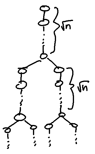
It seems that our complexity would be something like $$$O(n+q \log(\sqrt n) \log(\sqrt n))$$$, which has quite low constant compared to the implementation using a single segment tree on a normal balanced binary tree since $$$\log^2(\sqrt n) = \frac{1}{4} \log^2(n)$$$. Is there a tree that can make the constant higher?
Really Fast Segment Trees
When looking for fast segment tree implementations, most people would probably direct you to the AtCoder Library $$$[5]$$$ where they have implemented a fast lazy segment tree template with which maintains an array with elements in the monoid $$$S$$$ and is able to apply operation $$$F$$$ acting on $$$S \to S$$$ on an interval in the array. Although their code is very fast, we can speed it up by assuming that the functions are commutative. That is for $$$f,g \in F, x \in S, f(g(x))=g(f(x))$$$, which is usually true for the uses of segment trees in competitive programming.
There is actually a way to handle lazy tags in a way that does not change implementation of iterative segment tree too much. The idea is pretty similar to what is mentioned in $$$[6]$$$. We do not propagate lazy tags. Instead, the true value of a node in the segment tree is $$$val_u + \sum\limits_{v \text{ is ancestor of } u} lazy_v$$$ and we apply the lazy tags in a bottom-up fashion when doing queries.

Below is code for segment tree that handles range increment updates and range max queries.
Link-Cut Tree
Let's just maintain a link-cut tree with some modifications to the underlying splay tree. Specifically, we additionally store a value which is the composition of values in the subtree of the splay tree (we only consider those vertices in the same chain). To perform a query on $$$u$$$ to $$$v$$$ (WLOG $$$u$$$ has lower depth than $$$v$$$), perform $$$access(u)$$$ then $$$access(v)$$$. Let $$$w=lca(u,v)$$$. It is possible that $$$w=u$$$. The below image shows the state of the tree after performing $$$access(u)$$$ and $$$access(v)$$$ respectively.
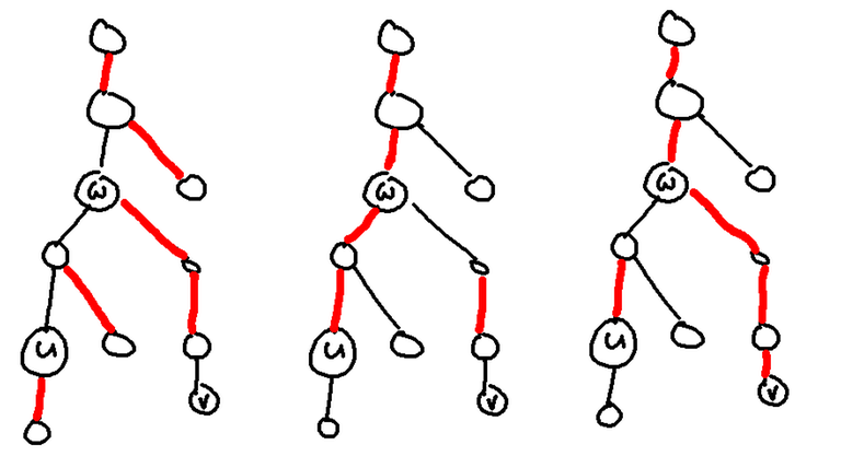
After performing both accesses, we would have $$$w$$$ being the root of the entire splay tree since we have accessed $$$u$$$ before $$$v$$$, $$$w$$$ would have already been in the same chain as the root before we start to access $$$v$$$. At the same time, we must splay $$$w$$$ when we are accessing $$$v$$$. So $$$w$$$ would be the last thing we splay, making it the root of the entire splay tree. Now, it is actually easy to perform path queries from $$$u$$$ to $$$v$$$. If $$$u=w$$$, then we simply query $$$w$$$ and the right child of $$$w$$$ (which is the path to $$$v$$$). If $$$u \neq w$$$, then we have to additionally include the path from $$$u$$$ to $$$w$$$ (but not including $$$w$$$). Luckily, due to the way we have accessed the vertices, this path would be exactly the chain containing $$$u$$$.
HLD + Splay Tree
Let's replace the segment tree in the HLD solution with a splay tree with the same modification to the underlying splay tree as the earlier section. If we need to query the prefix of a splay tree, just splay the vertex then additionally query the left child. If we need to query the subarray of $$$[l,r]$$$ on the splay tree, splay $$$l$$$ to the root and $$$r$$$ to just below root, then we only have to additionally query the right child of $$$r$$$. Remember for a HLD query, we do some prefix queries and at most $$$1$$$ subarray query.
What would be the complexity? It seems like it would be the same $$$O(n + q \log^2 n)$$$. But no, it can be shown that it is actually $$$O(n+q\log n)$$$. Yes, it is not a typo. I still don't believe it myself even though the justification is below.
In the same way we showed that access works in $$$O(\log n)$$$ in link-cut trees, we will do the same here by imagining that there are fake edges from the root of each chain of the splay tree to its the parent of the chain so when we define the rank function and count the number of vertices in a subtree of $$$u$$$, we also take into account those vertices connected via fake edges. It is not too hard to see that the time complexity for the path query between $$$a$$$ and $$$b$$$ would be a similar telescoping sum resulting in $$$O(r_{final}(a)+r_{final}(b)-r_{initial}(a)-r_{initial}(b)+k_a+k_b)=O(\log n)$$$.
Balanced HLD
Although the previous $$$2$$$ algorithms have $$$O(n+q\log n)$$$ complexity. They are extremely unpractical as splay trees (or any dynamic tree) carry a super huge constant. Is it possible to transfer the essence of what splay tree is doing into a static data structure?
What was so special about our HLD+splay tree solution that it is able to cut one log when compared to HLD+any other data structure? It's splaying! That is if a vertex was recently accessed, it would be pushed near to the root the tree even though it may have many light edges on its path to the root. This property of caring about the entire tree structure is unique to splay trees and isn't found in any other method mentioned here as other data structures treat each of the heavy chains independently.
So, we need to create a data structure that is similar to HLD+segment tree but instead of having a structure based on dividing based on the sum of weights of unweighted nodes (which is a segment tree), maybe let's give each node a weight and split the based on those weight. Wait, isn't that centroid decomposition?
Indeed, let us first do HLD then take the heavy chain containing the root of the tree. For each vertex in this heavy chain, give each vertex a weight which is the number of vertices in its connected components after removing all edges in the heavy chain. And that's pretty much the entire idea. Divide things based on the weighted case. More specifically, given a heavy chain with total weight $$$W$$$, choose a vertex $$$x$$$ such that the total weight of the left and rights sides of the chain (excluding $$$x$$$) have weight $$$\leq \frac{W}{2}$$$. Such a vertex always exists (it's the centroid). We set $$$x$$$ as the root of the binary tree and recurse on the left and right childs. For the subtrees that are children of the heavy chain, repeat this process and we have constructed our desired tree.
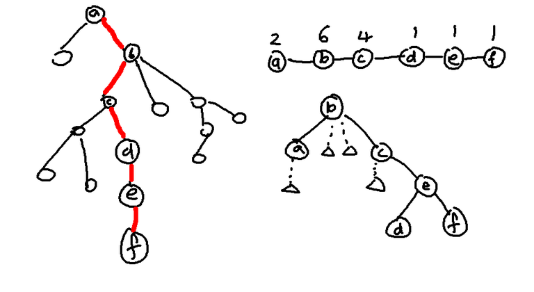
Now, we need to show that queries here are indeed $$$O(\log n)$$$. First we need to think about how we actually perform queries in our HLD structure. We know from HLD+segment tree our query loop is for querying the path between $$$a$$$ and $$$b$$$ is this:
- if $$$a$$$ and $$$b$$$ are in the same heavy chain, query $$$in[a]$$$ to $$$in[b]$$$
- if $$$a$$$ is deeper than $$$b$$$, query $$$in[hpar[a]]$$$ to $$$in[a]$$$
- if $$$b$$$ is deeper than $$$a$$$, query $$$in[hpar[b]]$$$ to $$$in[b]$$$
Of these $$$3$$$ queries, only the first query type is a sub-array query on the heavy chain, the rest of them are queries on prefixes of the heavy chain. Furthermore, the first query type is only done once. Now, what is the time complexity for a prefix query on a binary tree? It may be tempting to say it is "just $$$O(\log n)$$$ duh", but we can improve it.
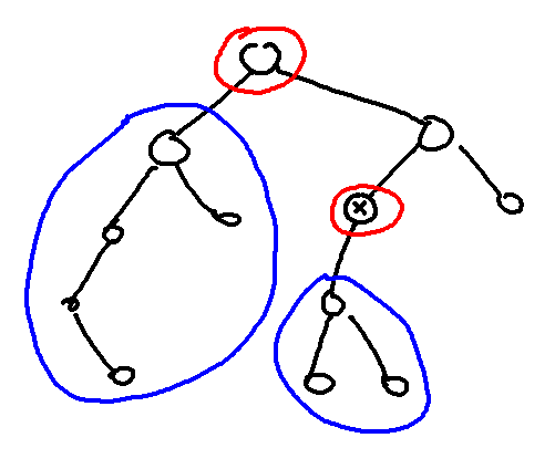
For example, if we want to query the values on the prefix where the last vertex is the one labelled $$$x$$$, we simply perform a walk from vertex $$$x$$$ to the root of the tree and add the costs of those vertices and their left children where appropriate (if we have walked up from the left child, don't add stuff). Walking from vertex $$$x$$$ to the root of the tree takes $$$O(d_x-d_{root}+1)$$$ time. For the case of sub-array queries on $$$[x,y]$$$ we can see that it is walking from $$$x$$$ and $$$y$$$ respectively to the root of the tree which will take $$$O(d_x+d_y-d_{root}-d_{root}+1+1)$$$.
Let's change the definition of $$$d_a$$$ slightly to be the depth when the consider the entire structure of our tree (so we consider light edges too when calculating the depth). Let $$$x_{root}$$$ be the root of the heavy chain containing vertex $$$x$$$. The time complexity for prefix or suffix queries becomes $$$O(d_x-d_{x_{root}}+1)$$$ and for sub-array queries it becomes $$$O(d_x+d_y-d_{x_{root}}-d_{y_{root}}+2)$$$. Then we can see that the time complexity is some telescoping sum here too, since when we traverse a light edge, the depth of the would decrease. Actually we don't need the telescoping sum justification here as we can just prove it by saying the querying the simple path from $$$x$$$ to $$$y$$$ only requires us to move $$$x$$$ and $$$y$$$ upwards (and never downwards). In the end, the time complexity only depends on the depth of the endpoints of our queries. So, the only thing we need to prove is that the depth of the entire tree is bounded by $$$O(\log n)$$$.
But the proof of that is exactly the proof that centroid decomposition gives us a centroid tree of depth at most $$$O(\log n)$$$. Maybe I should elaborate more. Let's consider the new tree structure we have built. There are $$$2$$$ types of edges, heavy edges and light edges. When we traverse down a heavy edge, the size of the subtree would be at least halved due to how we have chosen to split the heavy tree so there are most $$$O(\log n)$$$ heavy edges on the path from some vertex to the root on our constructed tree. However, when we traverse down a light edge, there is no guarantee about what happens to the size of the subtree, except it can decrease by $$$1$$$, which is pretty useless. Luckily for us, we know that for every vertex, it has at most $$$O(\log n)$$$ light edges on the path to the root, because that's how HLD works. So we can determine that the depth of the tree is $$$O(\log n)+O(\log n)=O(\log n)$$$. We have shown that our complexity for querying is $$$O(\log n)$$$. Also, is not too hard show that our complexity of construction of this structure is $$$O(n \log n)$$$ since constructing the tree from a single heavy chain is literally centroid decomposition.
The depth of the tree is $$$O(\log n)$$$ but what is the constant. The number of heavy and light edges are both $$$\log n$$$ so our analysis from earlier gives us a $$$2 \log n$$$ bound on the height of the tree. Can we do better? It turns out no, this bound is sharp (up to $$$\pm 1$$$ maybe). Here is how we can construct a tree that forces the depth to be $$$2 \log n$$$ by our construction.
Let $$$T(s)$$$ be our constructed tree that has $$$s$$$ vertices. It is defined recursively by the below image.
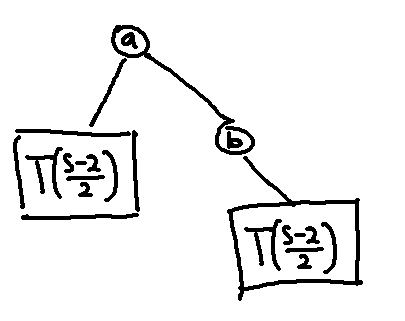
Let $$$d(s)$$$ denote the depth of $$$T(s)$$$. As a base case, $$$d(0)=0$$$. We also have $$$d(s)=2+d(\frac{s-2}{2})$$$ since the heavy chain of $$$T(s)$$$ would be on the right side of the tree, so $$$a$$$ would be connected to its left child by a light edge in the original tree. We can have the root of the heavy chain be vertex $$$b$$$ in our constructed tree (it can be vertex $$$a$$$ but we want to assume the worst case) so that in our construction tree, $$$a$$$ would have a depth of $$$2$$$, requiring us to traverse $$$2$$$ edges to get to $$$T(\frac{s-2}{2})$$$. Therefore, it is easy to see that we can make $$$T(s)$$$ have a height of about $$$2 \log n$$$.
Path and Subtree Queries
With our normal HLD+segment tree query, we can easily handle both path and subtree queries $$$[7]$$$.
Can we do it for our new structure? Yes.
Firstly, one of the problems of subtree operations is that if the number of children is very large, it will be hard to compute the aggregate values of children. This is the reason for the difficulty of $$$[9]$$$. But we are not doing operations on a dynamic tree, we can simply augment our tree to make the number of children small for our case.
As in $$$[9]$$$, the idea is to binarize the tree, however since we do not have to care about the depth of the augmented tree, we can simply augment it into a caterpillar graph.
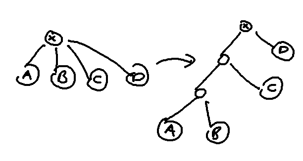
Subtree operations are the same on the original tree and the main tree. The only case we have to handle differently is path operations. For example, the path $$$A \to B$$$ passes through $$$X$$$ in the original tree but not in the augmented tree. However, we can solve this by checking if the lca of $$$A$$$ and $$$B$$$ is a fake vertex. If so, we separately process the actual lca in the original tree.
The original lazy tag we used when we only had path queries only applies the value to the children in the real tree. However with subtree queries, we need a new lazy tag that applies the value to all children, which includes children connected via light edges. Modifying the code to add another lazy tag is not hard, just very tedious.
More specifically, we have $$$2$$$ lazy tags, $$$lazy1$$$ and $$$lazy2$$$. $$$lazy1$$$ is applied to the children in the same heavy chain while $$$lazy2$$$ is applied to all children regardless of whether or not they are in the same heavy chain.
Then, the true value of a vertex $$$u$$$ in the balanced binary tree is $$$val_u + \sum\limits_{\substack{v \text{ is ancestor of } u \\ v \text{ and } u \text{ same heavy chain}} }lazy1_v + \sum\limits_{v \text{ is ancestor of } u }lazy2_v$$$.
Modifying these changes to the original algorithm is not difficult, just very tedious.
Benchmarks
Here are the benchmarks for the various implementations of the tree path queries so that you have a better ideas of the practical performance of the things I will describe so you will realize that the algorithm is practically pretty useless (except, maybe some interactives which are similar to $$$[8]$$$).
The problem is given a tree with $$$n=10^6$$$ vertices where all vertices initially of weight $$$0$$$, handle the following $$$q=5 \cdot 10^6$$$ operations of $$$4$$$ types:
1 u v wincrease the weights of all vertices on the simple path from $$$u$$$ to $$$v$$$ by $$$w$$$2 u vfind the maximum weight of any vertex on the simple path from $$$u$$$ to $$$v$$$3 u wincrease the weights of all vertices on the subtree of $$$u$$$ by $$$w$$$4 ufind the maximum weight of any vertex on the subtree of $$$u$$$
It is bench-marked on my desktop with Ryzen 7 3700X CPU with compilation command g++ xxx.cpp -O2.
Note that the difference between balanced HLD 1 and 2 is that balanced HLD 2 is able to handle all types of queries while balanaced HLD 1 is only able to handle the first $$$2$$$ queries.
Benchmarks when there are only query types $$$1$$$ and $$$2$$$.
| HLD + segment tree (single segment tree) | HLD + segment tree (many segment tree) | HLD + segment tree (many segment tree, ACL) | link-cut tree | HLD + splay tree | Balanced HLD 1 | Balanced HLD 2 | |
|---|---|---|---|---|---|---|---|
| Time Complexity | $$$O(n + q \log ^2 n)$$$ | $$$O(n + q \log ^2 n)$$$ | $$$O(n + q \log ^2 n)$$$ | $$$O(n+q \log n)$$$ | $$$O(n + q \log n)$$$ | $$$O((n + q) \log n)$$$ | $$$O((n+q) \log n)$$$ |
| Random ($$$wn=0$$$) | $$$14.31~s$$$ | $$$8.91~s$$$ | $$$10.89~s$$$ | $$$8.66~s$$$ | $$$9.77~s$$$ | $$$7.90~s$$$ | $$$13.38~s$$$ |
| Random ($$$wn=-10$$$) | $$$10.84~s$$$ | $$$6.65~s$$$ | $$$6.97~s$$$ | $$$5.78~s$$$ | $$$5.18~s$$$ | $$$4.54~s$$$ | $$$11.17~s$$$ |
| Random ($$$wn=10$$$) | $$$15.14~s$$$ | $$$10.73~s$$$ | $$$12.62~s$$$ | $$$10.69~s$$$ | $$$13.25~s$$$ | $$$10.04~s$$$ | $$$13.74~s$$$ |
| Binary Tree ($$$k=1$$$) | $$$21.45~s$$$ | $$$13.09~s$$$ | $$$17.49~s$$$ | $$$12.40~s$$$ | $$$13.62~s$$$ | $$$10.59~s$$$ | $$$13.96~s$$$ |
| Binary tree ($$$k=5$$$) | $$$20.48~s$$$ | $$$14.64~s$$$ | $$$18.12~s$$$ | $$$11.82~s$$$ | $$$15.16~s$$$ | $$$11.80~s$$$ | $$$14.90~s$$$ |
Benchmarks when there are all $$$4$$$ query types.
| HLD + segment tree (single segment tree) | Balanced HLD 2 | |
|---|---|---|
| Time Complexity | $$$O(n + q \log ^2 n)$$$ | $$$O((n+q) \log n)$$$ |
| Random ($$$wn=0$$$) | $$$9.06~s$$$ | $$$10.61~s$$$ |
| Random ($$$wn=-10$$$) | $$$7.12~s$$$ | $$$8.86~s$$$ |
| Random ($$$wn=10$$$) | $$$9.92~s$$$ | $$$11.15~s$$$ |
| Binary Tree ($$$k=1$$$) | $$$13.47~s$$$ | $$$11.80~s$$$ |
| Binary tree ($$$k=5$$$) | $$$11.67~s$$$ | $$$11.63~s$$$ |
I am unsure why a value of $$$k$$$ closer to $$$\sqrt n$$$ made the first $$$3$$$ codes all faster. Maybe there is something wrong with my generator or is the segment tree just too fast? Also, IO takes about $$$1~s$$$.
Here are my codes (generators + solutions). They have not been stress tested and are not guaranteed to be correct. They are only here for reference.
1/3 Centroid Decomposition
When I was writing this blog, I was wondering whether we could cut the $$$log$$$ factor from some centroid decomposition problems. Thanks to balbit for telling me about this technique.
Consider the following problem: You are given a weighted tree of size $$$n$$$ whose edges may have negative weights. Each vertex may either be toggled "on" or "off". Handle the following $$$q$$$ operations:
- Toggle vertex $$$u$$$.
- Given vertex $$$u$$$, find the maximum value of $$$d(u,v)$$$ over all vertices $$$v$$$ that is toggled "on". It is guaranteed that at least one such $$$v$$$ exists.
It is well-know how to solve this in $$$O(n \log n + q \log^2 n)$$$ by using centroid decomposition + segment trees. But can we do better?
The reason segment trees have to be used is because when we query for the longest path ending at some centroid parent to perform our queries, we have to ignore the contribution of our own subtree. An obvious way to solve this is to try to decompose the centroid tree in such a way that each vertex has at most $$$2$$$ children. Unfortunately, I do not know a way to do this such that the depth of the tree bounded by $$$\log_2 n$$$, but there is a way to make the depth of the tree bounded by $$$log_{\frac{3}{2}} n$$$.
Instead of thinking of doing centroid decomposition on vertices, let us consider doing it on edges. Top image is the usual cetroid decomposition, while bottom image is the one we want to use here. That is, the centroid gets passed down to its children when recursing.
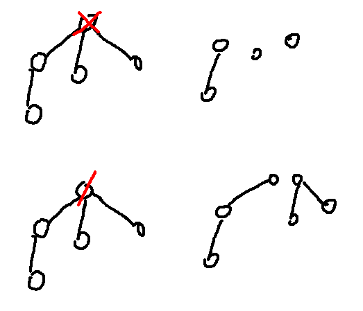
Ok, so now we want to figure out what is the largest possible number of edges of the smaller partition. Remember, we want to make this value as large as possible to get a split that is as even as possible.
Firstly, we have a lower bound $$$\frac{1}{3}m$$$, whre $$$m$$$ is the number of edges. This is obtained when the tree is a star graph with $$$3$$$ children. The number of edges in each subtree are $$$[1,1,1]$$$, it is clear that the best way to partition the subtrees is $$$[1]$$$ and $$$[1,1]$$$, which gives us our desired lower bound.
Now, we will show that this bound is obtainable. Let $$$A$$$ be an array containing elements in the interval $$$[0,\frac{1}{2}]$$$ such that $$$\sum A=1$$$. This array $$$A$$$ describes the ratio between the number of edges in each subtree against the total number of edges. The elements are bounded above by $$$\frac{1}{2}$$$ due to the properties of the centroid.
Then, the following algorithm surprisingly finds a subset $$$S$$$ whose sum lies in the range $$$[\frac{1}{3},\frac{2}{3}]$$$.
1. tot=0
2. S={}
3. for x in [1,n]:
4.     if (tot+A[x]<=2/3):
5.         tot+=A[x]
6.         S.insert(x)
It is clear that $$$\sum\limits_{s \in S} A[s] \leq \frac{2}{3}$$$, so it suffices to show that $$$\sum\limits_{s \in S} A[s] \geq \frac{1}{3}$$$.
Let $$$P[x]=A[1]+A[2]+\ldots+A[x]$$$, that is $$$P$$$ is the prefix sum array.
Consider the first index $$$x$$$ such that $$$P[x]>\frac{2}{3}$$$. We will split into $$$2$$$ cases.
- $$$A[x]<\frac{1}{3}$$$: when we have completed iteration $$$x-1$$$, the $$$\sum\limits_{s \in S} A[s] = P[x-1] = P[x]-A[x] > \frac{1}{3}$$$.
- $$$A[x] \geq \frac{1}{3}$$$: it is easy to see that the final $$$S=[1,n] \setminus \{x\}$$$. So $$$\sum\limits_{s \in S} A[s] = 1-A[x] \geq \frac{1}{2}$$$.
Therefore, we are able to obtain a centroid tree which is a binary tree and has depth at most $$$\log_{\frac{3}{2}} n$$$.
Returning back to the original problem, we are able to solve it in $$$O(n \log n + q_1 \log^2 n + q_2 \log n)$$$ where $$$q_1$$$ and $$$q_2$$$ are the number of queries of type $$$1$$$ and $$$2$$$ respectively.
References
[1] https://github.com/dawxy/ACM-CODER/blob/master/%E3%80%90%E8%AE%BA%E6%96%87%26%26%E6%95%99%E7%A8%8B%E3%80%91/QTREE%E8%A7%A3%E6%B3%95%E7%9A%84%E4%B8%80%E4%BA%9B%E7%A0%94%E7%A9%B6.pdf
[2] https://ocw.mit.edu/courses/6-854j-advanced-algorithms-fall-2008/921232cb9a69015c50002ff5ea6a9824_lec6.pdf
[3] https://courses.csail.mit.edu/6.851/spring12/scribe/L19.pdf
[4] https://en.wikipedia.org/wiki/Link/cut_tree
[5] https://codeforces.net/blog/entry/82400
[6] https://codeforces.net/blog/entry/72626
[7] https://codeforces.net/blog/entry/53170
[8] https://oj.uz/problem/view/JOI14_secret
[9] https://codeforces.net/blog/entry/103726


It seems everyone disagrees what the name of this technique should be. So let's settle it.
The trick is known in literature as Biased Binary Search Tree (BiBST), originated in Sleator's paper as far as I remembered.
Daniel Sleator is active on codeforces so maybe can just ask him? Ping Darooha
For the acronym alone, CBT.
When I was told about this technique, it was referred to as global BST (and not global HLD), so I prefer that name merely for convenience reasons. Not really sure where the "global" comes from, though.
Error-gone or Ara-gorn?
I did not understand this part. Why does it become O(n+qlogn) complexity if we have a segment tree for each heavy path?
He's saying it becomes $$$O(n+q\log n)$$$ only when the original tree is a binary tree, which should be pretty obvious since the sum of chain lengths is $$$\log n$$$. In the table further down it gives the general $$$O(n+q\log^2n)$$$
Oh, I missed that the sum of chain lengths is $$$ \log n $$$. Thank you very much.
for the 1/3 centroid decomposition, is it possible to construct a tree where you hit the 1/3,2/3 worst case for all decompositions?
for example for the 3-star tree, the first split is 1/3,2/3 but then you have 3 linked lists for which you can split 1/2,1/2 all the way down
for example you can solve this problem 1592D - Hemose in ICPC ? with 1/3CD as long as you choose your splits closely enough to 1/2,1/2 240284857