Recently I was learning about how to binary search over suffix array to solve string matching (specifically, single text, multiple patterns, solve it online). Here (1 ("Pattern Query" section), 2, 3) describes how to solve it in O(|s| * log(|p|)) but I'll describe how to improve this to O(|s| + log(|p|)). There already exists resources online about this, but I will try to simplify it.

visualizing suffix array

Let's take the text s="banana", and consider all suffixes (written vertically):

a
n a
a n a
n a n a
a n a n a
b a n a n a
0 1 2 3 4 5

now let's sort it:

      a
    a n
    n a   a
  a a n   n
  n n a a a
a a a b n n
5 3 1 0 4 2

s's suffix array is [5, 3, 1, 0, 4, 2].

Now take any substring of s (like "an"). Observe there exists a maximal-length subarray of s's suffix array ([3,1]) representing all the suffixes (3 -> "ana", 1 -> "anana") where "an" is a prefix. I like to call this the "subarray of matches": as this subarray represents all the starting indexes (in s) of a match.

Let's define a function which calculates this: subarray_of_matches(s[s_l:s_r]) = suffix_array[suffix_array_l:suffix_array_r].

Now observe that subarray_of_matches(s[s_l:s_r+1]) is nested inside subarray_of_matches(s[s_l:s_r]). This is because every spot where s[s_l:s_r+1] is a match, s[s_l:s_r] is also a match.

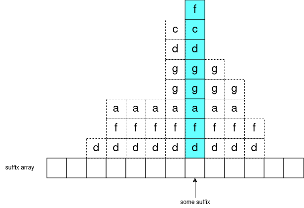
But in particular, we can take some suffix (like "anana") and plug in all of its' prefixes to subarray_of_matches and we get a sequence of nested subarrays:

subarray_of_matches("a") = [5,3,1]
subarray_of_matches("an") = [3,1]
subarray_of_matches("ana") = [3,1]
subarray_of_matches("anan") = [1]
subarray_of_matches("anana") = [1]

in general, you can visualize it like this:

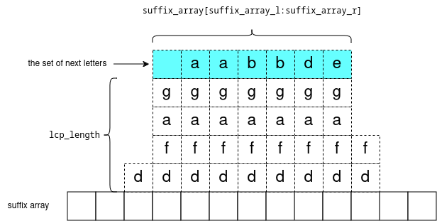
One more point: consider any subarray of the suffix array: suffix_array[suffix_array_l:suffix_array_r] and let lcp_length = the longest common prefix of these suffixes. Formally: for each i in range [suffix_array_l,suffix_array_r) the strings s[suffix_array[i]:suffix_array[i]+lcp_length] are all equal.

Now consider the set of next letters: s[suffix_array[i]+lcp_length], they are sorted. We can visualize it like:

visualizing the binary search

Given text s, s's suffix array, and query string p, our goal is to calculate the minimum index i such that p is a prefix of s[suffix_array[i]:] (the suffix of s starting at suffix_array[i])

so we can start the binary search as usual with l=0,r=size(s),m=(l+r)/2, and compare p to s[suffix_array[m]:]. if p is less, search lower (r=m;), else search higher (l=m;).

Let's also keep track of the "best" suffix so far, e.g. the suffix which matches the most characters in p. Let's store it as a pair {best_i_so_far,count_matched} with the invariant: p[:count_matched] == s[best_i_so_far:best_i_so_far+count_matched].

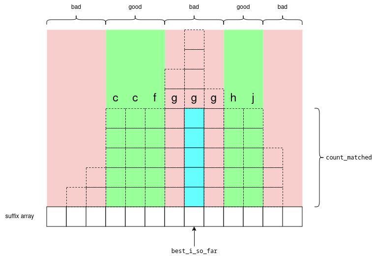
So now, depending on whether p[:count_matched+1] is less/greater than s[best_i_so_far:best_i_so_far+count_matched+1] we want to look for the green section which is before/after best_i_so_far. And here, we have the cases taken from here:

• the middle red section will not contain the answer because the pattern p didn't match with that letter g, so it still won't match anywhere in that range.

• the green sections will contain a match which is either better or the same as the middle red section

• the outer red sections won't contain the answer because the LCP is too low

So back to our binary search, we have l,r,m=(l+r)/2.

• If m lies in either of the red sections; then we can check for this in O(1) using a lcp query, and continue the search "towards" the green section.

• If m is already in the green section, then continue matching p[count_matched:] with s[best_i_so_far+count_matched:] (and also update our best match {best_i_so_far,count_matched})

we start comparing characters in p starting from count_matched, so we only compare characters in p once, and achieve complexity O(log(|s|) + |p|).

code: https://codeforces.net/edu/course/2/lesson/2/3/practice/contest/269118/submission/277693465