Section 1. Introduction

I have been struggling for weeks to understand the first linear-time planarity algorithm, the Hopcroft-Tarjan algorithm (HT). Fortunately, I successfully understood it and implemented it. In fact it is very hard to find a verified HT implementation online. Some code, e.g., LEDA is not open source. Other open-source planarity tests, e.g., networkx (LR planarity), boost (Boyer-Myrvold), Pigale (LR planarity), use other algorithms. There is an implementation by Shawn Anderson, however it is partial. I would like to open a blog to share my experience with Codeforces friends.

Definition: A graph is said to be planar if it can be drawn on the plane in such a way that its edges intersect only at their endpoints. There are two well known theorems for planar graphs:

(1)Kuratowski's theorem: A undirected simple graph is planar iff it contains neither a $$$K_{3,3}$$$-subdivision nor a $$$K_5$$$-subdivision.

(2)Wagner's theorem: A undirected simple graph is planar iff it contains neither $$$K_{3,3}$$$ nor $$$K_5$$$ as a minor.

Unfortunately, neither theorem yields an efficient algorithm. Enumerating $$$K_{3,3}$$$ or $$$K_5$$$ themselves is already very complicated. Besides, a graph that contains no $$$K_{3,3}$$$ and no $$$K_5$$$ might be non-planar, for example, take an arbitrary edge from $$$K_5$$$ (which has $$$10$$$ edges), and add $$$3$$$ points on the edge, leads to a non-planar graph. So, besides these two graphs themselves, we also need to enumerate the subgraphs that contain these two graphs as minors, making things much more difficult.

Let's switch back to HT. Given a graph $$$G$$$, we simplify $$$G$$$. First, self-loops and multiple edges do not infect planarity. We make the self-loops arbitrarily close to the vertices. If there are multiple edges between vertices $$$u$$$ and $$$v$$$, we can make them arbitrarily close, so only one of them needs consideration. Second, We can replace directed edges into undirected edges. The DFS tree of an undirected graph is simpler, it only contains two kinds of edges: Tree arcs and fronds (frond starts from a vertex $$$v$$$ and ends with an ancestor of $$$v$$$ in the DFS tree), while the DFS tree of a directed graph might contain tree arcs, fronds, and cross edges (a cross edge starts from a visited vertex $$$u$$$ to another visited vertex $$$v$$$, neither $$$u$$$ nor $$$v$$$ is an ancestor of the other). Third, it can be proved that if $$$|V| > 3$$$ then $$$|E| \leq 3|V| - 6$$$ (see Wikipedia). Therefore, $$$O(|V|) = O(|E|)$$$. If $$$|V| \leq 3$$$, $$$G$$$ is planar. If $$$|V| > 3$$$ and $$$|E| > 3|V| - 6$$$, we declare $$$G$$$ as non-planar without further investigation.

The most important simplification is turning this graph into bicomponents (bcc) (2-vertex-connected components). It is well known that a simple undirected graphs could be decomposed into a forest of bicomponents. So, $$$G$$$ is planar, iff all bccs of $$$G$$$ are planar. A bcc $$$B$$$ admits an ear decomposition. Formally speaking, $$$B$$$ could be obtained by the following process:

X := An initial Cycle C #(1)
while X != B:
    Add a path(*) starts from X and ends in X; #(2)

The path in (2), together with a path in X, forms a new cycle.

Tarjan's algorithm recursively consider these ears. Let's take the initial cycle $$$C$$$ as an example. By the Jordan curve theorem, $$$C$$$ separates the plane into two parts: The inner part and the outer part. The Jordan curve theorem is very difficult to prove, it involves profound algebraic topology prerequisites, called fundamental groups and homology groups, which I don't grasp. Fortunately, this theorem is very intuitively correct. Let's just use it. In fact, the Jordan curve theorem is the core reason HT uses BCCs. The inner part and outer part of $$$C$$$ lead to a very rough solution to planarity test & embedding: Consider the ears in $$$B-C$$$. We calculate the conflicts in these ears and model the conflicts as another graph $$$Conflict(B-C)$$$ whose vertices are these ears. If two ears in $$$B-C$$$ conflicts, we add an edge connecting them in $$$Conflict(B-C)$$$. If $$$Conflict(B-C)$$$ is bipartite, $$$B$$$ is planar, as we can throw one "color" into the cycle and leave another "color" outside the cycle. Below is an intuitive illustrate of the rough idea. However, there are many "details" not justified:

(1)How to represent an ear, which might contain multiple vertices & edges?

(2)For two ears in $$$Conflict(B-C)$$$, how can we tell whether they conflict?

(3)Even if we build the graph $$$Conflict(B-C)$$$, time complexity is another obstacle. In fact, there might be $$$O(|V|)$$$ such ears, so the conflict edges might be $$$O(|V|^2)$$$.

(4)There might be conflicts on other ears, not only on $$$C$$$. How should we deal with them?

Figure 1: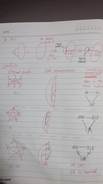

Figure 2: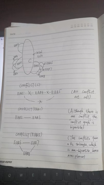

Section 2. The algorithm

We now answer the four questions in Section 1 one-by-one.

First, an ear is ($$$\geq 0$$$) tree arcs plus one frond. Note that an ear might be a single frond without any tree arc. Therefore, an ear is actually a path in the DFS tree (that's why HT has a pathfinder function and belongs to path addition category while there are many other categories, e.g., edge addition/edge deletion for planarity test). HT only cares about the start vertex and the end vertex of the ear (also known as a path), therefore storing the ears is easy. An question is that when we call pathfinder(v) (a pathfinder is also an ear finder, which essentially is a DFS procedure) and find an edge $$$v \rightarrow w$$$, how to tell whether $$$v \rightarrow w$$$ starts a new path or belongs to the old path? To answer this question, HT DFS twice. In the first round DFS, HT assigns each edge (might be a tree arc or a frond) with a non-negative value. How to define this value will be discussed later. pathfinder, which is the second round DFS, visit $$$w \in adj(v)$$$ by the ascending order of $$$value(v \rightarrow w)$$$, i.e., the edges with smaller value would be visited earlier than the edges with higher value. That is equivalent to sorting $$$adj(v)$$$ by value ascendingly. If $$$w$$$ is the first vertex in $$$adj(v)$$$, $$$v \rightarrow w$$$ inherits the old path, otherwise, $$$v \rightarrow w$$$, which might be a tree arc or a frond, is the first edge of a new path (ear). Note that if the value is bounded by $$$O(|V|)$$$, we can use $$$O(|V|)$$$ bucket sort instead of $$$O(|V|log|V|)$$$ quick/heap sort, so the sorting process is not a barrier to the linearity of the algorithm. The "Two DFS" is very similar to the heavy-light decomposition HLD (see CP-Algorithms, OIWIKI). Note that HT and HLD are two complemently different algorithms, however the "DFS twice trick" and "path decomposition" in both algorithms are similar.

Second, the HT paper detects the conflicts of two paths in its Lemma 9.

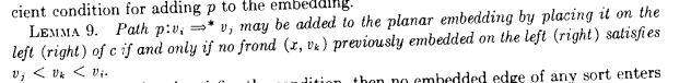
The readers might be confused about the suddenly appeared lemma. Don't worry, I will explain it. $$$vi \Rightarrow vj$$$ is just the path we discussed above ($$$\geq 0$$$ tree arcs plus a frond). The word "previously" indicates there is a sequence for finding paths. The sequence is, first explore the path, $$$v_1$$$, $$$v_2$$$, ..., $$$v_n$$$, where the first vertex of $$$adj(v_i)\,1 \leq i < n$$$ is $$$v_{i+1}$$$ and $$$v_i \rightarrow v_{i+1}$$$ is a tree arc. WLOG we assume that the first edge of $$$v_n$$$, say $$$v_n \rightarrow w$$$, is a frond (if not so, we can continue search $$$w$$$). When we call pathfinder(v_1), it first goes to $$$v_2$$$, then $$$v_3$$$, ... , then $$$v_n$$$, and finishes the path at $$$w$$$. The DFS number of the sequence satisfies $$$DFN(w) \leq DFN(v_1) < DFN(v_2) < ... < DFN(v_n)$$$. The reason why $$$DFN(w) \leq DFN(v_1)$$$ is due to the 2-vertex-connectivity of the graph, and $$$DFN(w) = DFN(v_1)$$$ iff $$$v_1$$$ belongs to the initial cycle. If the value of edges are properly defined and correctly calculated, $$$DFN(w) < DFN(v_1)$$$ always holds. The calculation of edge value will be discussed later. When the pathfinder algorithm reaches $$$v_n$$$, it starts to pathfinder (note that pathfinder is a recursion) other ears starting $$$v_n$$$ and finds some fronds. After finishing the exploration of $$$v_n$$$, it starts exploring $$$v_{n-1}$$$, $$$v_{n-2}$$$, ..., $$$v_2$$$ in the reversed order of the DFS number! Also, Tarjan tends to use the word "may" in his paper. Actually, the words "may" in his paper means "confirmly can". So, let's reformulate Lemma 9 in our words:

A path $$$v_i$$$->(tree arcs)->$$$a$$$--(frond)->$$$b$$$ has a conflict with path $$$v_k\,(k > i)$$$->(tree arcs)->$$$c$$$--(frond)->$$$d$$$ iff $$$DFN(b) < DFN(d) < DFN(v_i)$$$. Since $$$k > i$$$ and the paths are generated in the reverse order of DFS numbers, the path starts with $$$v_k$$$ is previously generated.

Figure 3:

The intuitive conflict in the rightdown corner of Figure 3 demonstrates the easiest case of Tarjan's Lemma 9. However, there are more cases. There might be two paths emanating from the same $$$v_i$$$ (See (b) in Figure4), say $$$p$$$ := $$$v_i$$$ -> $$$a$$$ -> ... -> $$$v_j$$$ and $$$q$$$ := $$$v_i$$$ -> $$$b$$$ -> ... -> $$$v_k$$$. Suppose $$$DFN(v_j) < DFN(v_k)$$$, we needs to pathfind $$$p$$$ earlier than $$$q$$$. If not so, $$$q$$$ is explored earlier than $$$p$$$, when we explore $$$p$$$, $$$q$$$ becomes a so-called "previouly embedded path" contains $$$v_k$$$ satisfies $$$DFN(v_j) < DFN(v_k) < DFN(v_i)$$$. The algorithm would falsely "find" a conflict, however there is no conflict between $$$p$$$ and $$$q$$$ at all, see Figure 4. So we need to sort the edges $$$v \rightarrow w$$$ by $$$LOW(w)$$$ ascendingly. $$$LOW$$$, a.k.a, lowlink, is a very common and widely used in the tarjan's BCC and SCC algorithms, see Wikipedia, USACO, OIWIKI. We assume readers are familar with Tarjan's BCC and SCC algorithms. Even dumb guys like me know them well, I believe you can.

Figure 4: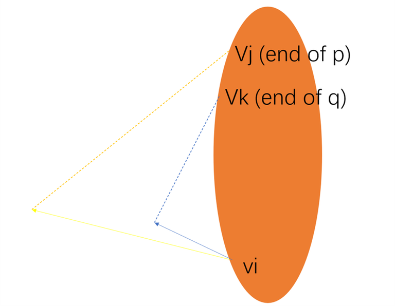

Also, there is a case we need to care about, and this is the only case we needs to use LOW2. That is, two paths might have the same starting $$$v_i$$$ and ending vertices $$$v_j$$$. That is Fig6(c) in the HT paper, and Figure 5 in our blog:

Figure 5: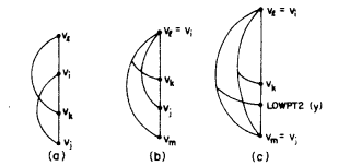

In such case, even if $$$x$$$ --> $$$v_k$$$ is a frond, there might be no conflict, if you ignore the LOWPT2(y) edge. So, we need to guarantee that, if a previously embedded path has a frond $$$x$$$ --> $$$v_k$$$ satisfies $$$DFN(v_j) < DFN(v_k) < DFN(v_i)$$$, the more recently generated path also has a frond $$$y$$$ --> $$$v_k^{'}$$$ satisfies that $$$DFN(v_j) < DFN(v_k^{'}) < DFN(v_i)$$$. However, the LOW value of these two paths are the same, both equal to $$$DFN(v_i)$$$. Therefore, it is necessary to introduce LOW2:

Let $$$S_v$$$ be the set of vertices such that $$$v$$$ could reach $$$S_v$$$ by $$$\geq 0$$$ tree arcs and a single frond. It is well known that $$$LOW(v) := min(DFN(\{v\} \cup S_v)\}$$$, and we define the LOW2 as $$$LOW2(v) := min(DFN(\{v\} \cup (S_v - LOW(v)))\}$$$. In the Figure5(c) case, a previously generated path also has a frond $$$y$$$ --> $$$v_k$$$ satisfies that $$$DFN(v_j) < DFN(v_k) < DFN(v_i)$$$ indicates that the LOW2 of the previous path is less than $$$DFN(v_i)$$$, although the LOW2 of that path might not be exactly $$$v_k$$$ (it might contain other fronds with DFN value less than $$$v_k$$$, but we don't care, we only care whether such $$$v_k$$$ frond exists or not). Therefore, if the LOW2 of the previous path is less than $$$DFN(v_i)$$$, we must force the LOW2 of the lately generated path less than $$$DFN(v_i)$$$. Therefore, the score of edge could be defined as:

We then answer the third and the fourth question left in Section 1. The basic idea of HT is, when we finish searching a path $$$x$$$, we try to embed it on the outer (The paper uses L and R instead of outer and inner), if there are two previously-embedding path $$$p \in outer$$$ and $$$q \in inner$$$ conflict with the current path $$$x$$$, the graph is non-plannar. Otherwise if there are only outer paths conflict with $$$x$$$, move these outer paths to inner. However, when paths are moved from outer to inner, some inner paths might also have to move outside! We call the connected components of the conflict graph as "blocks". The definition "blocks" also appear in the HT paper, which says: "Let a block B be a maximal set of entries on L (outer) and R (inner) which correspond to fronds such that the placement of any one of the fronds determines the placement of all the others". The definition of "blocks" is very important but hard to understand, so we offer some examples:

Figure 6: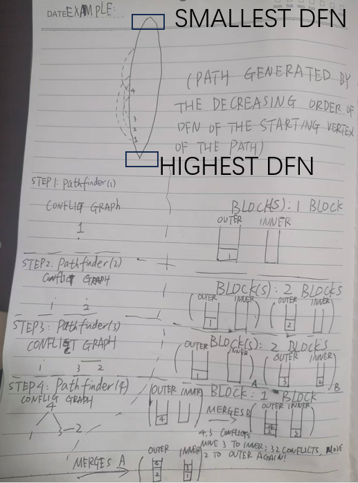

Figure 7: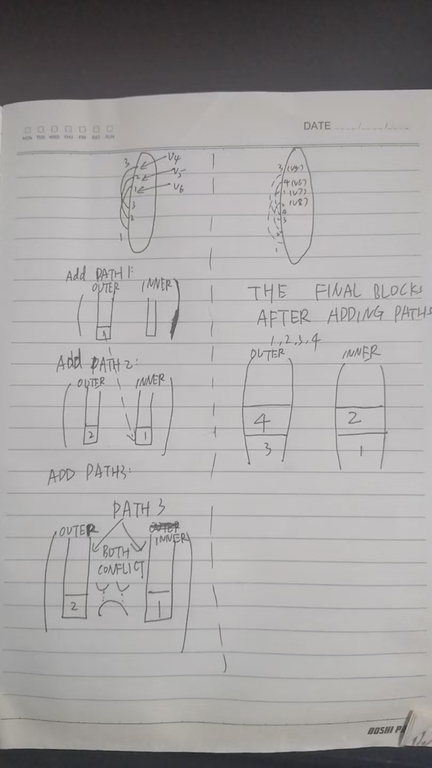

There are still two issues: The first one is the complexity issue, since a path might be switched from outer and inner multiple times. For examples, in Figure 6, PATH 2 is initially at outer when it is first explored. Then PATH 2 is switched to inner at STEP3, a.k.a, pathfinder(3), and then switched back to outer again in STEP 4 (pathfinder(4)). The complexity seems to blow up to quadratic, since we might flip $$$1+2+...+ O(|V|) = O(|V|^2)$$$ paths flipped in the iterations. The second issue is that the blocks might come from other ears, how can we distinguish them?

Let's imagine how the algorithm works. In fact, we don't store pathid into the blocks. Instead we store the DFN of the ending vertex of the paths. Note that if we store the DFN, there might be duplicated value in the blocks, as different paths might end with the same vertices. However, that does not infect the linearity of the complexity, even if there are duplicated DFN, the total number of them does not exceed**** the total number of paths, which is at most $$$|E| \leq 3|V| - 6$$$. Before we explore $$$v_i$$$, we need to delete all paths ending with $$$v_k$$$ such that $$$DFN(v_k) \geq DFN(v_i)$$$. When we explore $$$v_i$$$, we find fronds end with $$$v_j$$$. If $$$v_j$$$ and $$$v_i$$$ is in the same ear (well, how to distinguish whether they are in the same ear is a problem, the HT paper uses a end-of-stack marker which seems difficult), and there is an element $$$v_k \in $$$ Block $$$B$$$ such that $$$DFN(v_j) < DFN(v_k)$$$, then surely $$$DFN(v_j) < DFN(v_k) < DFN(v_i)$$$ holds, the reason why $$$DFN(v_k) < DFN(v_i)$$$ is that we have already deleted the paths with ending vertices $$$v_k$$$ such that $$$DFN(v_k) \geq DFN(v_i)$$$. According to Lemma 9, a conflict is found.

Figure 8: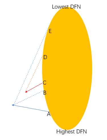

Let's take Figure 8 as an example. As we stressed above, the paths are explored by the descending order of the DFN value of the
starting vertex. The real line denotes a starting edge, while the dash lines are fronds. We first explore A, however, A itself is not recorded in any block, because we only record ending vertices of paths into blocks, while A is only a starting vertex. The algorithm records B and E into one block, both on the outer side. When the algorithm starts pathfinding C, since B has higher DFN value than C, B would be deleted from the blocks, while E would not be deleted before staring pathfinder(C). The deletion process make the outer (inner) entries of each block continuous (this is Lemma 10 in the HT paper). The word continuous is, if there are two entries $$$x, y$$$ in the outer of a block $$$B$$$, and $$$DFN(x) < DFN(y)$$$, then any entry $$$z$$$ satisfies $$$DFN(x) < DFN(z) < DFN(y)$$$, must belong to $$$B$$$. It could be proved that if $$$z$$$ belongs to the outer of $$$B_1 \neq B$$$, then the outer of $$$B_1$$$ and $$$B$$$ must conflict, so $$$B_1$$$ and $$$B$$$ should be one block instead of two. HT used two paragraphs to prove Lemma 10, however this lemma is very simple and intuitive, so we encourage the readers to prove themselves or refer to the paper. Well, I know codeforcers are very good at guessing, see Zhtluo's guess is all you need. I think Lemma 10 is only DIV2{B, C} level if you use some guessing, but it is indeed very important, and the proof is slightly hard to describe in words. We notice that, the deleting process could be fulfilled in linear time. By amortized analysis, we only add $$$O(|E|) = O(|V|)$$$ paths, so we only need to delete that many paths, although we might delete multiple paths in one step.

[A]We simulate the outer and inner of a block using two monotonic stacks. The top has the highest DFN value, while the bottom has the lowest DFN values. When we merge two blocks $$$B$$$ and $$$B_1$$$, we need to check $$$2 \times 2 = 4$$$ possible conflicts:

(1)[SameSide] $$$B$$$'s outer conflicts with $$$B_1$$$'s outer;

(2)[DiffSide] $$$B$$$'s outer conflicts with $$$B_1$$$'s inner;

(3)[DiffSide] $$$B$$$'s inner conflicts with $$$B_1$$$'s outer;

(4)[SameSide] $$$B$$$'s inner conflicts with $$$B_1$$$'s inner;

When checking whether a newly generated $$$B$$$ conflicts with an elder block $$$B_1$$$, by Lemma 9 in the HT paper, we only needs to consider whether $$$B_1.\{outer, inner\}.max > B.\{outer, inner\}.min$$$. The logic is

//mergeoldpath in our implementation
//B is a newly created block,  with a single frond in its outer, and B's inner is originally empty
while(previous_blocks.size())
{
    B1 = previous_blocks.back(); //an elder block
    bool sameside = ((1) holds [B_1.outer.max > B.outer.min] || (4) holds [B_1.inner.max > B.inner.min]); 
    bool diffside = ((2) holds [B_1.inner.max > B.outer.min] || (3) holds [B_1.outer.max > B.inner.min]);
    if(sameside && diffside) goto non-planar;
    if(!sameside && !diffside) 
    {
        break; //By the continuity of blocks, no need to check later
    }
    previous_blocks.pop_back();
    if(sameside) 
    { 
        //Same side confliction implies different side non-confliction
        //Otherwide, sameside && diffside==true and the algorithm won't come to this if branch!
        B.outer.concatenate(B1.inner);
        B.inner.concatenate(B1.outer);
    }
    else
    {
        B.outer.concatenate(B1.outer);
        B.inner.concatenate(B1.inner);
    }
}
//B becomes a "previously block"
previous_blocks.push_back(B);

Figure 9: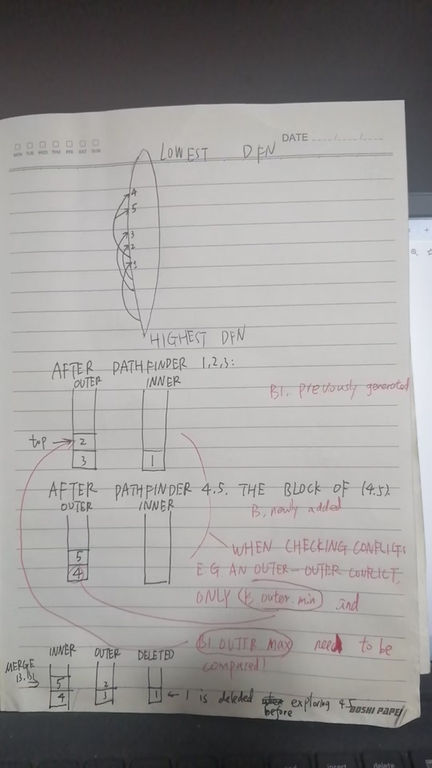

Therefore, we need a data structure that enables max(), min() and concatenate(another object of the same data structure). Well, that is a deque implemented using a single linked list! We always insert the elements from the front, and maintain the head, tail, nextptr and size correctly. When merging two linked lists, we just pointer the nextptr of the tail of one list to the other one!

[B] There is the last issue: How to distinguish different ears? In fact, there is one key difference between the additional ears and original cycle illustrated in the Figure 10. The shared path prevents some vertices from moving inside to outside. See Figure 10 for a demo.

Figure 10: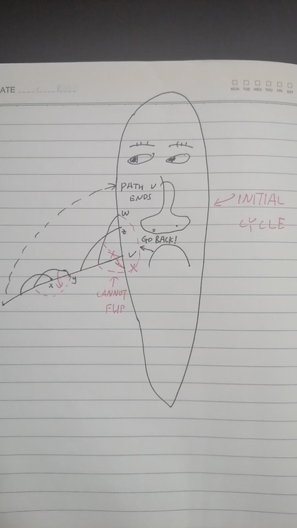

How to handle this issue? When the pathfinder function finishes that path, we don't need to consider vertices $$$x, y$$$ in Figure 10, so delete them from the block. For a block with ending vertices in the shared path, e.g., $$$w$$$ and $$$z$$$, only one of $$$outer$$$ and $$$inner$$$ from that block could contain the vertices in the shared path. If both $$$outer$$$ and $$$inner$$$ contains vertices in the shared path, the $$$outer$$$, $$$inner$$$, and the ear from the last call, form a "impossible triangle". This logic is implemented in mergenewblocks in our code.

Figure 11: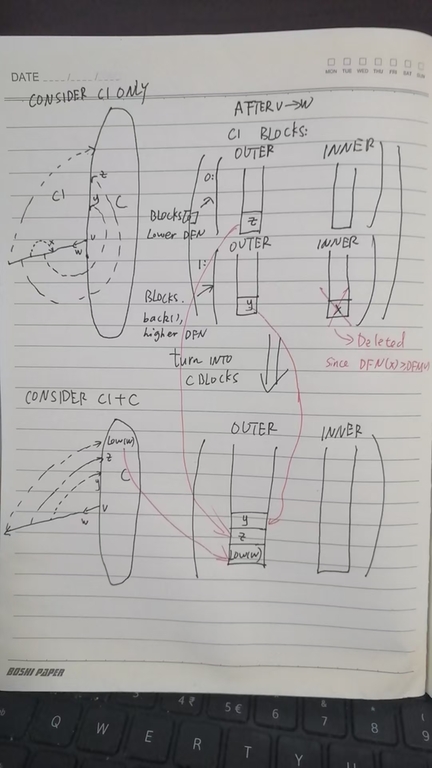

When we finish search $$$Path(v \rightarrow w)$$$, say $$$C_1$$$, we need to switch the blocks of $$$C_1$$$ to the blocks of $$$C$$$, say Figure 11. From the $$$C_1$$$ perspective, there might be multiple blocks, each of them can choose which side to stay. When it comes from $$$C_1$$$ back to say, they have to stay at the same side of $$$C$$$, therefore should be merged into one block.

Section 3. Implementation

Code is here:

#include <bits/stdc++.h>

int64_t getTimeStamp()
{
    std::chrono::time_point<std::chrono::system_clock,std::chrono::milliseconds> tp = std::chrono::time_point_cast<std::chrono::milliseconds>(std::chrono::system_clock::now());
    auto tmp=std::chrono::duration_cast<std::chrono::milliseconds>(tp.time_since_epoch());
    return (int64_t)tmp.count();
}

struct node
{
    node* next;
    int val;
};

std::vector<node*> newed;

struct mylist
{
    node* _head, *_tail; 
    int _size;
    mylist():_size(0)
    {
        _head = new node;
        newed.push_back(_head);
        _head->val = 0;
        _head->next = NULL;
        _tail = _head;
    }

    int front()
    {
        if(!_head || !_head->next)
        {
            return 0;
        }
        return _head->next->val;
    }

    int back()
    {
        if(_head == _tail || _tail == NULL) return 0;
        return _tail->val;
    }

    void push(int x)
    {
        node* tmp = new node;
        newed.push_back(tmp);
        tmp -> val = x;
        tmp -> next = _head->next;
        _head->next = tmp;
        ++_size;
        if(_size == 1) 
        {
            _tail = tmp;
        }
    }

    bool pop()
    {
        node* tmp = _head->next;
        if(!tmp || !_size) return false;
        _head->next = tmp->next;
        --_size;
        if(!_size)
        {
            _tail = _head;
        }
        return true;
    }

    int size()
    {
        return _size;
    }

    bool conc(mylist& another) //conc: concatenate [two lists]
    {
        if(!another._head) return false;
        if(another._size == 0)
        {
            another._head = NULL;
            return true;
        }
        _size += another._size;
        _tail -> next = another._head->next;
        _tail = another._tail;
        another._head = NULL;
        return true;
    }

    std::string debug()
    {
        std::stringstream ss;
        node* n = _head->next;
        while(n)
        {
            char buf[20] = {0};
            sprintf(buf, "%p", n);
            ss << n->val << "(" << buf << ") ";
            n = n->next;
        }
        return ss.str();
    }

    //There is no ~mylist DTOR here. It involves O(n) operations. So we do it in the last GC
};

struct B //blocks
{
    mylist l, r;
    B()=default;
    B(int x) { l.push(x); }
    void merge(B& another, int diff)
    {
        if(diff)
        {
            l.conc(another.r);
            r.conc(another.l);
        }
        else
        {
            l.conc(another.l);
            r.conc(another.r);
        }
    }

    std::string debug()
    {
        return std::string("l: ") + l.debug() + ", r: " + r.debug();
    }
};

struct G
{
    int _n, _m, _s, _p, _debug;
    std::vector<std::vector<int>> _o;
    std::vector<int> _f, _path;
    bool _planar;
    G(int n): _n(n), _m(0), _debug(0)
    {
        _o.resize(n+1);
        _path.resize(n+1);
    }

    void blocktrimmer(std::vector<B>& blocks, int v)
    {
        int removedl = 0, removedr = 0;
        while(!blocks.empty())
        {
            B& back = blocks.back();
            removedl = 0, removedr = 0;
            while(back.l.front() >= v) back.l.pop(), ++removedl;
            while(back.r.front() >= v) back.r.pop(), ++removedr;
            if(back.l.size() + back.r.size() == 0) blocks.pop_back();
            if(!removedl && !removedr) break;
        }
    }

    std::pair<B, bool> mergenewblocks(std::vector<B>& newblocks, int fw)
    {
        B ret;
        bool findfw = false;
        while(!newblocks.empty())
        {
            B& back = newblocks.back();
            if(back.l.front() > fw && back.r.front() > fw)
            {
                if(_debug)
                {
                    printf("[mergenewblocks return false]l.front():%d, r.front():%d, fw: %d, back:%s\n", 
                        back.l.front(), back.r.front() ,fw, back.debug().c_str());
                }
                return {ret, false};
            }
            if(back.l.front() == fw || back.r.front() == fw) findfw = true;
            if(back.l.front() > fw)
            {
                ret.l.conc(back.l);
            }
            else if(back.r.front() > fw)
            {
                ret.l.conc(back.r);
            }
            newblocks.pop_back();
        }
        if(_debug)
        {
            printf("[mergenewblocks]fw: %d, findfw: %d\n", fw, findfw);
        }
        if(findfw) 
        {
            B tmp(fw);
            ret.l.conc(tmp.l);
        }
        return {ret, true};
    }

    bool mergeoldpath(std::vector<B>& oldblocks, B& newblock)
    {
        while(!oldblocks.empty())
        {
            B& back = oldblocks.back();
            bool samesideinterlace = false;
            bool diffsideinterlace = false;
            if(back.l.size() && newblock.l.size() && back.l.front() > newblock.l.back())
            {
                samesideinterlace = true;
            }
            if(back.r.size() && newblock.r.size() && back.r.front() > newblock.r.back())
            {
                samesideinterlace = true;
            }
            if(back.l.size() && newblock.r.size() && back.l.front() > newblock.r.back())
            {
                diffsideinterlace = true;
            }
            if(back.r.size() && newblock.l.size() && back.r.front() > newblock.l.back())
            {
                diffsideinterlace = true;
            }
            if(!samesideinterlace && !diffsideinterlace)
            {
                break;
            }
            else if(samesideinterlace && diffsideinterlace)
            {
                if(_debug)
                {
                    printf("[mergeoldpath]back: %s, newblock: %s\n", back.debug().c_str(), newblock.debug().c_str());
                }
                return false;
            }
            else
            {
                newblock.merge(back, samesideinterlace);
                oldblocks.pop_back();
            }
        }
        if(newblock.l.size() > 0 || newblock.r.size() > 0)
        {
            oldblocks.push_back(newblock);
        }
        return true;
    }

    std::string BlockInfo(std::vector<B>& blocks)
    {
        std::stringstream ss;
        ss << "================BEGIN================\n";
        int i = 1;
        for(B& b: blocks)
        {
            ss << i << "/" << blocks.size() << ": " << b.debug() << "\n";
            ++i;
        }
        ss << "================END==================\n";
        return ss.str();
    }

    bool pathfinder(int v, std::vector<B>& blocks)
    {
        if(_debug) printf("[pathfinder entrance]v: %d[_path %d]\n", v, _path[v]);
        int i = 0;
        bool alreadyfindfrond = false;
        for(int w: _o[v])
        {
            ++i;
            if(i > 1) ++_p;
            if(w > v)
            {
                //tree arc
                _path[w] = _p;
                std::vector<B> newblocks;
                if(!pathfinder(w, _path[w] == _path[v] ? blocks : newblocks)) return false;
                if(_debug)
                {
                    printf("[pathfinder v%d(_path:%d)->w%d(_path:%d)]before blocktrimmer(\n[%s], %d), assign _path[%d] := %d\n", 
                        v, _path[v], w, _path[w], 
                        BlockInfo(_path[w] == _path[v] ? blocks : newblocks).c_str(), v, w, _p);
                }
                blocktrimmer(_path[w] == _path[v] ? blocks : newblocks, v);
                if(_debug)
                {
                    printf("[pathfinder v%d(_path:%d)->w%d(_path:%d)]after blocktrimmer(\n[%s], %d)\n", v, _path[v], w, _path[w], 
                        BlockInfo(_path[w] == _path[v] ? blocks : newblocks).c_str(), v);
                }
                if(_path[w] != _path[v])
                {
                    if(_debug)
                    {
                        printf("[pathfinder v%d->w%d]before mergenewblocks(\n[%s], %d)\n", v, w, 
                            BlockInfo(newblocks).c_str(), _f[_path[v]]);
                    }
                    auto [merged, canbeplanar] = mergenewblocks(newblocks, _f[_path[w]]);
                    if(_debug)
                    {
                        printf("[pathfinder v%d->w%d]after mergenewblocks(\n[%s], %d)-INTO>%s\n", v, w, 
                            BlockInfo(newblocks).c_str(), _f[_path[v]], merged.debug().c_str());
                    }
                    if(!canbeplanar) return false;
                    if(_debug)
                    {
                        printf("[pathfinder1 v%d->w%d]before mergeoldpath(\n[%s], [%s])\n", v, w, 
                            BlockInfo(blocks).c_str(), merged.debug().c_str());
                    }
                    canbeplanar = mergeoldpath(blocks, merged);
                    if(_debug)
                    {
                        printf("[pathfinder1 v%d->w%d]after mergeoldpath(\n[%s], [%s]), canbeplanar %d\n",
                            v, w, BlockInfo(blocks).c_str(), 
                            merged.debug().c_str(), canbeplanar);
                    }
                    if(!canbeplanar) return false;
                }
            }//tree arc
            else
            {
                alreadyfindfrond = true;
                _f[_p] = w;
                B b(w);
                if(_debug)
                {
                    printf("[pathfinder2 v%d-->w%d]before mergeoldpath(\n[%s], [%s]), assign _f[%d]: %d\n", v, w, 
                        BlockInfo(blocks).c_str(), b.debug().c_str(), _p, w);
                }
                bool canbeplanar = mergeoldpath(blocks, b);
                if(_debug)
                {
                    printf("[pathfinder2 v%d-->w%d]after mergeoldpath(\n[%s], [%s]) canbeplanar%d\n", v, w, 
                        BlockInfo(blocks).c_str(), b.debug().c_str(), canbeplanar);
                }
                if(!canbeplanar) return false;
            }
        } //end for, traverse all edges
        if(_debug) printf("[pathfinder returns true]v: %d[_path %d], blocks:\n[%s]\n", v, _path[v], BlockInfo(blocks).c_str());
        return true;
    }

    bool HopcroftTarjan()
    {
        if(!_debug)
        {
            if(_n <= 3) return true;
            if(_m > 3*_n - 6) return false;
        }
        _f.resize(_m+1); //m is updated outside
        _p = 0;
        _path[1] = 1;
        std::vector<B> blocks;
        return pathfinder(1, blocks);
    }

    bool HopcroftTarjanWrapper()
    {
        if(!HopcroftTarjan())
        {
            if(_debug) printf("%s\ncannot be planar!\n", EdgeInfoInFormat().c_str());
            return false;
        }
        return true;
    }

    std::string EdgeInfo()
    {
        std::stringstream ss;
        int sz = 0;
        for(int i = 1; i <= _n; ++i) sz += _o[i].size();
        for(int i = 1, j = 1; i <= _n; ++i)
        {
            for(int x: _o[i])
            {
                ss << "[" << j++ << "/" << sz << "]" << i << "->" << x << "\n";
            }
        }
        return ss.str();
    }

    std::string EdgeInfoInFormat()
    {
        std::stringstream ss;
        int sz = 0;
        for(int i = 1; i <= _n; ++i) sz += _o[i].size();
        ss << 1 << "\n" << _n << " " << _m << "\n";
        for(int i = 1, j = 1; i <= _n; ++i)
        {
            for(int x: _o[i])
            {
                ss << i << " " << x << "\n";
            }
        }
        return ss.str();
    }
};

bool HopcroftTarjan(std::vector<G>& bicomps)
{
    for(G& bcc: bicomps) if(!bcc.HopcroftTarjanWrapper()) return false;
    return true;
}

struct Gtmp{
    int _n, _idx, _m, _debug;
    std::vector<std::vector<int>> _o;
    std::vector<std::vector<std::pair<int, int>>> _buckets;
    std::vector<int> _low1, _low2, _dfn, _pa;
    Gtmp()=delete;
    Gtmp(int n, bool debug): _n(n), _idx(0), _m(0), _debug(debug)
    {
        _o.resize(_n+1);
        _buckets.resize(2*_n+2);
        _low1.resize(_n+1);
        _low2.resize(_n+1);
        _dfn.resize(_n+1);
        _pa.resize(_n+1);
    }

    void dfs(int v, int fa)
    {
        _dfn[v] = _low1[v] = _low2[v] = ++_idx;
        for(int w: _o[v])
        {
            if(!_dfn[w])
            {
                _pa[w] = v;
                dfs(w, v);
                _low1[v] = std::min(_low1[v], _low1[w]);
            }
            else if(w != fa)
            {
                _low1[v] = std::min(_low1[v], _dfn[w]);
            }
        }

        for(int w: _o[v])
        {
            auto vw = std::make_pair(v, w);
            if(_pa[w] == v) 
            {
                if(_low1[v] != _low1[w]) _low2[v] = std::min(_low2[v], _low1[w]);
                _low2[v] = std::min(_low2[v], _low2[w]);
                if(_low2[w] >= _dfn[v])
                {
                    _buckets[2*_low1[w]].push_back(vw);
                }
                else 
                {
                    _buckets[2*_low1[w]+1].push_back(vw);
                }
            }
            else if(_dfn[w] < _dfn[v] && w != fa)
            {
                if(_low1[v] != _dfn[w]) _low2[v] = std::min(_low2[v], _dfn[w]);
                _buckets[2*_dfn[w]].push_back(vw);
            }
        }
    }

    G operator()()
    {
        _idx = 0;
        for(int i = 1; i <= _n; ++i) _dfn[i] = 0;
        dfs(1, 0);
        G g(_n);
        g._debug = _debug;
        for(int i = 1; i <= 2*_n+1; ++i)
        {
            for(const auto& [v, w]: _buckets[i])
            {
                g._o[_dfn[v]].push_back(_dfn[w]);
                g._m++;
            }
        }
        return g;
    }
};

struct GraphToBiconnectedComponents
{
    GraphToBiconnectedComponents() = delete;
    GraphToBiconnectedComponents(int n): _n(n), _m(0), _debug(false){
        _o.resize(n+1); _bccids.resize(n+1); _rename.resize(n+1);
    }
    int _n;
    int _top;
    int* _low;
    int* _dfn;
    int* _s;
    int _idx;
    int _m;
    bool _debug;
    int _test;

    std::vector<std::vector<int>> _o, _bccs;
    //_rename: _rename each biconnected component as 1, 2, ...
    //This is definitely not a necessary step in the HT algorithm, however,
    //it makes every biconnected component more `independent` and `easier to debug`.
    std::vector<int> _bccids, _rename; 
    std::set<std::pair<int, int>> st; //It is O(log n), never mind, it is not very important

    int add_edge(int u, int v)
    {
        if(u == v) return -1;
        if(u < 1 || u > _n) return -3;
        if(v < 1 || v > _n) return -4;
        auto uv = std::make_pair(u, v);
        if(st.count(uv)) return -2;
        st.insert(uv);
        st.insert(std::make_pair(v, u));
        _o[u].push_back(v);
        _o[v].push_back(u);
        ++_m;
        return 0;
    }

    void tarjan(int u, int fa)
    {
        int son = 0;
        _low[u] = _dfn[u] = ++_idx;
        _s[++_top] = u;
        for(int v: _o[u])
        {
            if(!_dfn[v])
            {
                ++son;
                tarjan(v, u);
                _low[u] = std::min(_low[u], _low[v]);
                if(_low[v] >= _dfn[u])
                {
                    _bccs.push_back(std::vector<int>{});
                    while(_s[_top+1] != v)
                    {
                        _bccs.back().push_back(_s[_top--]);
                    }
                    _bccs.back().push_back(u);
                }
            }
            else if(v != fa) _low[u] = std::min(_low[u], _dfn[v]);
        }
        if(fa == 0 && son == 0) //isolated point
        {
            _bccs.push_back(std::vector<int>{});
            _bccs.back().push_back(u);
        }
    }

    std::vector<G> calc(bool debug, int test)
    {
        std::vector<G> biconnected;
        if(_n > 3 && _m > 3*_n - 6) return biconnected;
        _bccs.clear();
        _low = new int[_n+1];
        _dfn = new int[_n+1];
        _s = new int[_m+_n+1];
        memset(_low, 0, (_n+1)*sizeof(int));
        memset(_dfn, 0, (_n+1)*sizeof(int));
        memset(_s, 0, (_m+_n+1)*sizeof(int));
        _idx = 0;
        _test = test;
        for(int i = 1; i <= _n; ++i)
        {
            if(_dfn[i]) continue;
            _top = 0;
            tarjan(i, 0);
        }

        int bccid = 1;
        for(const std::vector<int>& bcc: _bccs)
        {
            int i = 1;
            Gtmp gtmp((int)bcc.size(), debug);
            //bcc is slightly different from scc: A vertex might belong to multiple bccs
            for(int x: bcc) 
            {
                _bccids[x] = bccid;
                _rename[x] = i++;
            }
            for(int x: bcc)
            {
                for(int y: _o[x])
                {
                    if(_bccids[x] == _bccids[y])
                    {
                        gtmp._o[_rename[x]].push_back(_rename[y]);
                        gtmp._m++;
                    }
                }
            }
            assert(gtmp._m%2 == 0);
            gtmp._m /= 2; //Handshake lemma of graph degree
            ++bccid;
            biconnected.push_back(gtmp());
        }
        delete[] _low;
        delete[] _dfn;
        delete[] _s;

        return biconnected;
    }
};

struct InputHelper
{
    std::vector<G> receiveoneinput(int test, bool luoguHNOI2010P3209=false, bool debug=true)
    {
        int n, m;
        scanf("%d %d", &n, &m);
        GraphToBiconnectedComponents biconnection_helper(n);
        for(int i = 1, u = 0, v = 0; i <= m; ++i)
        {
            scanf("%d %d", &u, &v);
            int res = biconnection_helper.add_edge(u, v);
            if(res == -1 && debug)
            {
                printf("[%d edge %d m %d]u:%d, v: %d, n: %d, m: %d, self loop!\n", test, i, m, u, v, n, m);
            }
            else if(res == -2 && debug)
            {
                printf("[%d edge %d m %d]u:%d, v: %d, n: %d, m: %d, duplicate!\n", test, i, m, u, v, n, m);
            }
            else if(res == -3 && debug)
            {
                printf("[%d edge %d m %d]u:%d, v: %d, n: %d, m: %d, u out of range!\n", test, i, m, u, v, n, m);
            }
            else if(res == -4 && debug)
            {
                printf("[%d edge %d m %d]u:%d, v: %d, n: %d, m: %d, v out of range!\n", test, i, m, u, v, n, m);
            }
            else if(debug) 
            {
                printf("[%d edge %d m %d]%d<-->%d\n", test, i, m, u, v);
            }
        }
        //The luogu https://www.luogu.com.cn/problem/P3209 problem provides a Hamilton cycle,
        //however we don't use them.
        for(int i = 1, u = 0; luoguHNOI2010P3209 && i <= n; ++i)
        {
            scanf("%d", &u); //We don't use `u`.
        }
        std::vector<G> components = biconnection_helper.calc(debug, test);
        return components;
    }

    std::vector<std::vector<G>> operator()(bool multitest, bool luoguHNOI2010P3209=false, bool debug=true)
    {
        std::vector<std::vector<G>> ans(1);
        int t = 1, test = 1;
        if(multitest)
        {
            scanf("%d", &t);
        }
        while(t--)
        {
            ans.push_back(receiveoneinput(test++, luoguHNOI2010P3209, debug));
        }
        return ans;
    }
};

int main(void)
{
    int64_t start = getTimeStamp();
    int debug = false;
    int luogu = true;
    std::vector<std::vector<G>> res = InputHelper()(true /*multitests*/, luogu /*luoguHNOI2010P3209*/, debug /*print*/);
    for(int i = 1; i < res.size(); ++i) 
    {   
        if(debug) 
        {
            printf("HopcroftTarjan: test case %d/(%zu in total), res[%d] size %zu", i, res.size()-1, i, 
                res[i].size()
            );
            int j = 1;
            for(G& bicomp: res[i])
            {
                printf("%d[testcase id]/%d[testcases]/%d[bicompid]/%d[bicomps] bicomp:\n%s\n", 
                    i, res.size()-1, j, res[i].size(), bicomp.EdgeInfo().c_str());
                printf("%s\n", bicomp.EdgeInfoInFormat().c_str());
                ++j;
            }
        }
        printf((res[i].size() && HopcroftTarjan(res[i]))?"YES\n":"NO\n");
    }
    for(node* x: newed) delete x;
    int64_t end = getTimeStamp();
    if(!luogu) printf("%lld\n", end-start);
}

If you set debug=true in the main function, the algorithm will print the detail. However, the running time is no longer linear, because it requires some $$$O(|V|)$$$ traversal at some steps. There is a variable called int luogu. If luogu is true, the program receives the Luogu P3209 type input: First it will read an integer $$$t$$$ indicating the number of test cases. Then, for each of the $$$t$$$ cases, the program receives the number of vertices $$$n$$$ and number of edges $$$m$$$. In the following $$$m$$$ lines, the program receives $$$m$$$ undirected edges. Finally, Luogu P3209 guarantees that the graph contains a Hamiltonian cycle, and provides us with this cycle. Our program hence receives $$$n$$$ numbers indicating the Hamiltonian cycle, however, we don't use this Hamiltonian cycle. For each of $$$t$$$ testcases, the program outputs YES if it is planar, or NO if it is non-planar. The program is tested on Luogu with verdict AC time 164ms.

Also we test some stronger cases. If luogu is false, we don't the $$$n$$$ numbers. Other inputs are the same. See this in the code:

for(int i = 1, u = 0; luoguHNOI2010P3209 && i <= n; ++i)
{
    scanf("%d", &u); //We don't use `u`.
}

For the output part, we output an additional line indicating the running time in millisecond. This is checked by comparing with networkx in Python. The test code is below. Note that I save the C++ code as ht.cpp and compile like g++ ht.cpp -o ht -g -Ofast, with luogu==false and debug==false (these two are necessary). If the answer of my implementation is different from that of networkx implementation, then the Python checker would assert(false). However, when you see this assert(false), please first check whether your compiled version has luogu==false please. The Python checker generates Erdos-Renyi graphs for testing, and the max edge probability is proportional to the reciprocal of the number of vertices, to make the expectation of the number of edges to be a linear function of the number of vertices. Well, if the graph contains too many edges, it is sure to output "NO", and we cannot test the pathfinder, which is the core part of the algorithm.

import random, os, networkx
#https://github.com/satemochi/is_planar
from is_planar import is_planar

def gen(nplist):
    length = len(nplist)
    s = "%s\n"%length
    ans = []
    totaln = 0
    glist = []
    i = 0
    for n, p in nplist:
        totaln += n
        #print("gen: i:%s, lennp:%s, totaln:%s"%(i, len(nplist), totaln))
        i += 1
        g = networkx.erdos_renyi_graph(n, p)
        glist.append(g)
        b = "YES" if is_planar(g) else "NO" #may call networkx.is_planar(g), but the networkx implementation is slower
        ans.append(b)
        edges = g.edges
        s += "%s %s\n"%(n, len(edges))
        for x, y in edges:
            s += "%s %s\n"%(x+1, y+1)
    return s, ans, totaln, glist

def turngraphintostr(g):
    edges = g.edges
    s = "1\n"
    s += "%s %s\n"%(len(g.nodes), len(edges))
    for x, y in edges:
        s += "%s %s\n"%(x+1, y+1)
    return s

def doonetest():
    for game in range(35):
        nplist = []
        for n in range(30, 220):
            for p in range(5, 2000//n):
                nplist.append((n, p/100))
        print("game:%s, nplist len:%s"%(game, len(nplist)))
        s, ans, totaln, glist = gen(nplist)
        print("game:%s, after gen, nplist len:%s, glist len:%s, totaln:%s"%(game, len(nplist), len(glist), totaln))
        with open("test1.txt", "w") as f:
            f.write(s)
        with os.popen("ht.exe < test1.txt") as f:
            l = f.readlines()
        l = list(map(lambda x: x.strip(), l))
        if len(l) < len(ans) or len(ans) != len(glist):
            print("lenwa: %s, lenac: %s"%(len(l), len(ans)))
            assert(False)
        print("game:%s, nplist len:%s, lenwa:%s, lenac:%s"%(game, len(nplist), len(l), len(ans)))
        for i in range(len(ans)): #len(l) might > len(ans), because ht.exe might print time consumption info
            if ans[i] != l[i]:
                print('i:', i, 'WA:', l[i], 'AC:', ans[i])
                print('i:', i, 'graph:\n', glist[i])
                print(turngraphintostr(glist[i]))
                assert(False)
        if len(l) > len(ans):
            print("game:%s, totaln:%s, Time consumed by ht.cpp in milliseconds:%s"%(game, totaln, l[len(ans)]))

def testone(s):
    lines = s.split('\n')
    t = int(lines[0])
    i = 1
    while t > 0:
        g = networkx.Graph()
        n, m = list(map(int, lines[i].strip().split()))
        i += 1
        for node in range(n):
            g.add_node(node)
        for edge in range(m):
            x, y = list(map(int, lines[i].strip().split()))
            i += 1
            g.add_edge(x-1, y-1)
        print("YES" if networkx.is_planar(g) else "NO")
        print("[DEBUG]YES" if is_planar(g) else "[DEBUG]NO")
        t -= 1

def testonefromfile(file):
    with open(file, "r") as f:
        x = f.read()
    testone(x)
    

if __name__ == '__main__':
    doonetest()
    #testonefromfile("test1.txt")

Our implementation is, first check the $$$|E| \leq 3|V| - 6$$$ condition, if not satisfied, directly output NO(Non-planar). Otherwise, use the class Gtmp to do the first DFS, compute DFN, LOW, and LOW2. Gtmp also (bucket) sorts the edges, and construct BCCs represented by the struct G. In G, to make the program more concise, the DFN order is equal to the vertex order (this is fulfilled using g._o[_dfn[v]].push_back(_dfn[w]);). Then, each BCC is independent to each other, and has a root, say $$$1$$$. For each BCC, we check the $$$|E| \leq 3|V| - 6$$$ condition again. If satisfied, we perform pathfinder(1) on that BCC. In the era of two algo giants Hopcroft and Tarjan, RAM resource is rather low so they need to carefully design the algorithms, and such design might sacrifice the readability of the code. Another reason might be that they are $$$998244353$$$ times clever than me, so I found their code, especially EMBED(G), very hard to understand. Therefore, I implement it myself. The blocks are clearlier represented, and no end-of-stack marker is needed. Also, the merging of blocks seems also clearer. The $$$[A]$$$ merging (search $$$[A]$$$ marker in Section 2) is implemented in mergeoldpath, and the $$$[B]$$$ merging is implemented in mergenewblocks. The second parameter of mergenewblocks is the lowest end of the shared path. This function is called after we search $$$v \rightarrow w$$$ where $$$w$$$ starts a new path different than $$$v$$$, therefore $$$v$$$ is the highest end of the shared path. The deleting process is implemented in blocktrimmer(std::vector<B>& blocks, int v). It will delete the elements in blocks with DFN value $$$\geq DFN(v)$$$. My implementation takes $$$3.5s$$$ on $$$250186$$$ vertices without any optimization, and if you enable -Ofast, it is about $$$2s$$$ on $$$250186$$$ vertices, with a normal Intel-I7 computer.